In the landscape of deep learning, models are typically designed to predict a target variable $y$ given an input $\mathbf{x}$. Autoencoders, however, subvert this paradigm. At their core, an autoencoder is a neural network trained to reproduce its own input, effectively learning to approximate the identity function $f(\mathbf{x}) \approx \mathbf{x}$.

While training a network to act as a simple “copy machine” might sound mathematically trivial, the true power of an autoencoder lies in its architectural constraints. By forcing the input data through a low-dimensional bottleneck before reconstructing it, the network is restricted from simply memorizing the input space. Instead, it is compelled to learn a compact, informative representation of the data’s underlying continuous manifold. This compressed latent representation serves as a powerful foundation for a multitude of advanced downstream tasks.

1.1. The Autoencoder Concept

Autoencoders belong to the broader family of self-supervised learning architectures. In these systems, the supervision signal is derived inherently from the data itself rather than from expensive, human-annotated labels. The network learns to predict missing or transformed parts of the data from the remaining parts.

In the specific case of an autoencoder, the “missing part” is the entirety of the original input. By minimizing the reconstruction error between the input data and the output prediction, the network naturally learns to encode the most salient features necessary for faithful reconstruction, discarding noise and redundant information in the process.

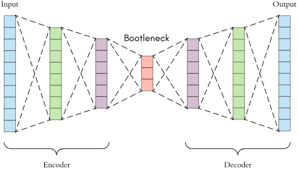
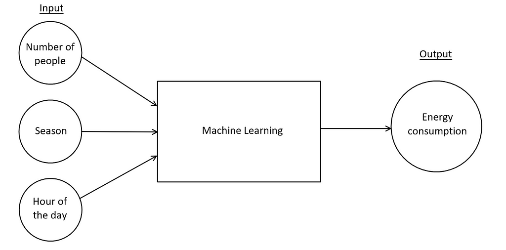
Figure 1 – High-level conceptual diagram of an autoencoder, illustrating the input mapping to a compressed latent code and expanding back to the reconstructed output [1].

1.2. Primary Objectives

The motivation behind deploying autoencoders generally falls into three primary objectives:

• Dimensionality Reduction and Manifold Learning: Similar to classical linear techniques like Principal Component Analysis (PCA), autoencoders learn a compressed representation that captures the intrinsic variance of a dataset in far fewer dimensions. However, because neural networks utilize non-linear activation functions, autoencoders can successfully model complex, non-linear data manifolds that linear hyperplanes cannot capture.
• Denoising and Robust Representation: By intentionally corrupting input data (e.g., adding Gaussian noise) and training the network to reconstruct the original, uncorrupted signal, we create a Denoising Autoencoder. This forces the model to learn features that are invariant to small perturbations, effectively projecting noisy data back onto the true data manifold—an essential property for robust perception and sensor pipelines.
• Feature Extraction for Downstream Tasks: The latent space—the narrowest point of the network—acts as a repository of highly abstracted features. Once an autoencoder is trained, the encoder half can be detached and used as an unsupervised feature extractor. These rich, low-dimensional embeddings can drastically improve the performance and convergence speed of subsequent classification, clustering, or visualization tasks.

1.3. Article Structure

Beyond basic reconstruction, the autoencoder framework serves as a conceptual bridge between traditional representation learning and modern generative modeling. This article will deconstruct the architecture, implementation, and evolution of autoencoders. The progression is organized as follows:

• Section 2 formalizes the core architecture and mathematical foundations, detailing the precise mappings of the encoder, the geometry of the latent space, and the probabilistic interpretation of reconstruction loss functions.
• Section 3 examines the MLP Autoencoder, illustrating how fully connected layers handle unstructured data, accompanied by a foundational PyTorch implementation.
• Section 4 extends these principles to image data via the CNN Autoencoder, highlighting the necessity of spatial coherence and convolutional downsampling.
• Section 5 bridges theory and practice by exploring real-world applications, with a deep dive into using reconstruction error for unsupervised anomaly detection.
• Section 6 introduces the generative extension: the Variational Autoencoder (VAE). We will explore how injecting probabilistic inference and the reparameterization trick into the latent space laid the groundwork for today’s advanced generative AI models.

2. Core Architecture and Mathematical Foundations

At the heart of every autoencoder lies a simple but powerful premise: a neural network can learn to compress information and subsequently reconstruct it. This is achieved through a tripartite architecture composed of an encoder, a latent space (or bottleneck), and a decoder. Each component plays a distinct functional role in transforming high-dimensional input data into a lower-dimensional manifold and then projecting it back to the original input space.

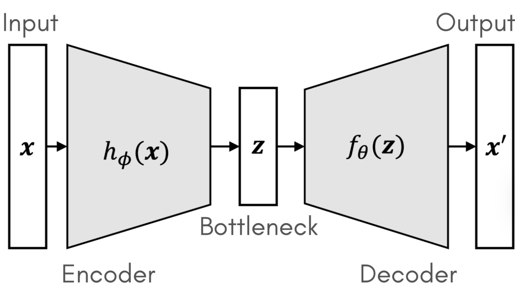
Figure 2 – Detailed schematic of encoder, bottleneck, decoder, and loss feedback [2].

2.1. The Encoder Mapping

The encoder is a deterministic mapping function, typically parameterized by a neural network, that compresses the input vector into a latent representation.

Let the input data be denoted as $\mathbf{x} \in \mathbb{R}^D$. The encoder function $f_{\theta}(\cdot)$, parameterized by weights and biases $\theta$, maps the input to a latent vector $\mathbf{z} \in \mathbb{R}^d$:

For a standard feedforward layer, this operation can be expanded as $\mathbf{z} = \sigma(\mathbf{W} \mathbf{x} + \mathbf{b})$, where $\mathbf{W}$ is the weight matrix, $\mathbf{b}$ is the bias vector, and $\sigma(\cdot)$ is a non-linear activation function (such as ReLU or GeLU). The encoder’s objective is to capture the most salient, invariant features of the data distribution while systematically discarding noise and redundancy.

2.2. The Latent Space (Bottleneck)

The latent space, often referred to as the bottleneck, is the compressed internal representation carrying the structural essence of the input. Its dimensionality, $d$, dictates the information capacity of the network.

Geometrically, the latent space can be interpreted as a low-dimensional manifold embedded within the high-dimensional input space $\mathbb{R}^D$. By forcing the network to route all information through this restrictive bottleneck $(d < D)$, we prevent it from trivially memorizing the data. Instead, the network must learn the intrinsic coordinates of this manifold, ensuring that each point $\mathbf{z}$ corresponds to a distinct, structurally valid reconstruction.

2.3. The Decoder Mapping

The decoder performs the inverse geometric transformation, projecting the low-dimensional latent codes back into the original, high-dimensional input space.

Denoted as $g_{\phi}(\cdot)$ and parameterized by $\phi$, the decoder maps the latent vector $\mathbf{z}$ to a reconstructed output $\hat{\mathbf{x}} \in \mathbb{R}^D$:

Together, the encoder and decoder form a composite function. The network’s success is determined by how closely the reconstruction $\hat{\mathbf{x}} = g_{\phi}(f_{\theta}(\mathbf{x}))$ mirrors the original input $\mathbf{x}$.

2.4. Reconstruction Loss Functions: A Probabilistic Perspective

Training an autoencoder involves minimizing a reconstruction loss $\mathcal{L}(\mathbf{x}, \hat{\mathbf{x}})$. While standard implementations treat this as a simple error metric, it is fundamentally grounded in Maximum Likelihood Estimation (MLE). The choice of loss function implies a specific probabilistic assumption about the underlying data distribution.

• Mean Squared Error (MSE) and the Gaussian Assumption: MSE is the default choice for continuous data. Minimizing the MSE is mathematically equivalent to maximizing the log-likelihood of the data, assuming the decoder’s output defines the mean of a multivariate isotropic Gaussian distribution with fixed variance.

• Binary Cross-Entropy (BCE) and the Bernoulli Assumption:If the input features are binary or normalized to the [0, 1] interval (e.g., pixel intensities), BCE is the mathematically correct objective. BCE assumes the targets are drawn from a multivariate Bernoulli distribution, treating the decoder’s output as the parameter (probability) of that distribution.

2.5. Undercomplete vs. Overcomplete Networks

Autoencoders are categorized by the relationship between the input dimension $D$ and the latent dimension $d$:

• Undercomplete Autoencoders ($d < D$): This is the standard configuration. The strict bottleneck naturally forces dimensionality reduction and feature extraction without requiring explicit regularization.
• Overcomplete Autoencoders ($d \ge D$): When the latent space is larger than or equal to the input space, the network possesses enough capacity to learn a trivial identity mapping ($f(\mathbf{x}) = \mathbf{x}$) without extracting meaningful features. To prevent this, overcomplete models require strict mathematical constraints:
  • Sparse Autoencoders: Introduce a sparsity penalty (e.g., an L1 regularization term or a Kullback-Leibler divergence penalty) on the latent activations. This forces the model to represent inputs using only a small, specialized subset of active neurons, learning highly localized features.
  • Contractive Autoencoders: Penalize the sensitivity of the latent representation to small variations in the input. This is achieved by adding the Frobenius norm of the encoder’s Jacobian matrix to the loss function: $\lambda \|\nabla_{\mathbf{x}} f_{\theta}(\mathbf{x})\|_F^2$. This explicitly forces the manifold to be robust against local perturbations.

2.6. Training Procedure

Despite being an unsupervised algorithm, an autoencoder is trained using the standard supervised learning machinery—the only difference is that the input $\mathbf{x}$ acts as its own target label.

The optimization loop proceeds as follows:

1. Forward Pass: Compute the latent representation $\mathbf{z} = f_{\theta}(\mathbf{x})$ and the reconstruction $\hat{\mathbf{x}} = g_{\phi}(\mathbf{z})$
2. Loss Calculation: Evaluate the objective function $\mathcal{L}(\mathbf{x}, \hat{\mathbf{x}})$, augmented with any regularization terms (e.g., sparsity or contractive penalties).
3. Backward Pass: Backpropagate the error gradients $\nabla_{\theta, \phi} \mathcal{L}$ through the decoder and then through the encoder using the chain rule.
4. Parameter Update: Adjust the weights $\theta$ and $\theta \phi$using gradient-based optimizers such as Adam or Stochastic Gradient Descent (SGD).

Each layer is followed by a non-linear activation function, such as ReLU, to introduce expressive capacity. The final decoder layer typically uses a Sigmoid activation when input data are normalized to the [0, 1] range.

Finding the right latent size is therefore a balance between compression efficiency and reconstruction quality. This trade-off is typically explored empirically through experiments on validation data.

3. The Multilayer Perceptron (MLP) Autoencoder

The Multilayer Perceptron (MLP) autoencoder is the most fundamental instantiation of the autoencoder family. Built exclusively from fully connected (dense) layers, this architecture treats input data as flat, one-dimensional vectors. While it is the standard choice for tabular datasets, sensor arrays, or low-dimensional continuous signals, examining its application to image data reveals both the core principles of representation learning and the inherent limitations of feedforward networks.

3.1. Architectural Overview

An MLP autoencoder dictates that every neuron in a given layer is connected to every neuron in the subsequent layer. The architecture symmetrically scales down the input into the latent space and then scales it back up.

Consider a standard baseline task: reconstructing grayscale images from the MNIST dataset. An original $28 \times 28$ pixel image is first flattened into a vector $\mathbf{x} \in \mathbb{R}^{784}$. The network architecture sequentially compresses this vector:

• Encoder Pathway: $\mathbb{R}^{784} \to \mathbb{R}^{128} \to \mathbb{R}^{64} \to \mathbb{R}^{32}$
• Latent Space ($\mathbf{z}$): A 32-dimensional bottleneck.
• Decoder Pathway: $\mathbb{R}^{32} \to \mathbb{R}^{64} \to \mathbb{R}^{128} \to \mathbb{R}^{784}$

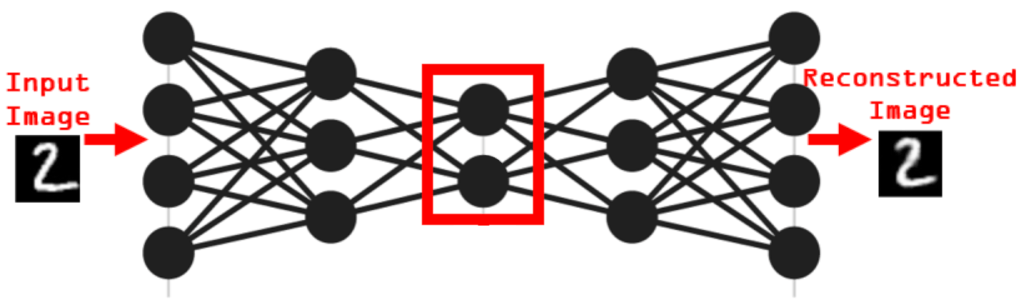
Figure 3: Example structure of an MLP autoencoder and sample reconstructions for the MNIST dataset. The left column shows input digits; the right column shows reconstructed outputs [3]

Each intermediate layer applies a non-linear activation function, such as ReLU ($f(x) = \max(0, x)$), to learn complex, non-linear mappings. The final layer of the decoder typically applies a Sigmoid activation ($f(x) = \frac{1}{1 + e^{-x}}$) to constrain the reconstructed pixel values strictly within the $[0, 1]$ range, matching the normalized input distribution.

3.2. Bottleneck Sizing: The Compression Trade-off

The dimensionality of the latent space is the most critical hyperparameter in an MLP autoencoder. It governs a strict trade-off between compression efficiency and reconstruction fidelity:

• Aggressive Compression (Small d): Enforces a tight informational bottleneck. The network is forced to learn only the most dominant eigenvectors (or their non-linear equivalents) of the data distribution. While excellent for anomaly detection and noise reduction, overly aggressive compression results in severe underfitting, leading to highly blurred or generalized reconstructions.
• Loose Compression (Large d): Preserves more variance from the input. While this minimizes the reconstruction loss ($\mathcal{L}_{\text{rec}}$), it increases the risk that the network will learn redundant features or default to a trivial identity mapping, effectively memorizing the training set without extracting generalizable structural rules.

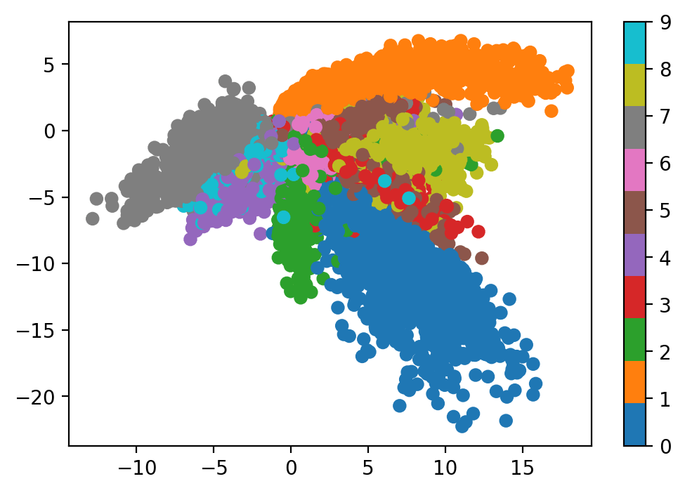
Figure 4 – Latent space visualization. By projecting the 32-dimensional latent vectors down to 2D using t-SNE or UMAP, we can observe how the autoencoder naturally clusters similar structural inputs, such as digits of the same class, without any label supervision.

3.3. PyTorch Implementation

The following code provides a robust, minimal implementation of an MLP autoencoder in PyTorch using nn.Sequential blocks. This structure emphasizes the symmetry between the encoder and decoder.

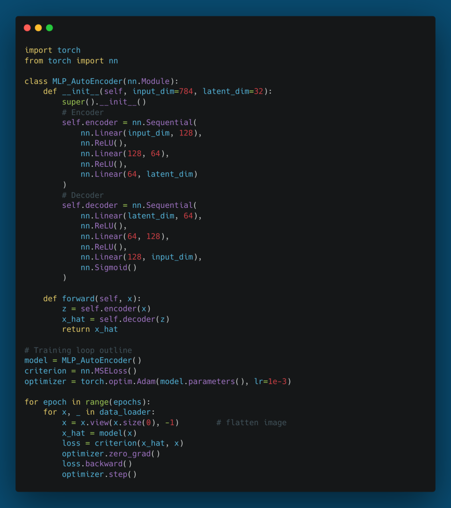
3.4. Reconstruction Quality and Spatial Limitations

When trained on visually simple datasets like MNIST, the MLP autoencoder successfully learns to reconstruct the inputs. However, a critical analysis of the outputs reveals a distinct blurriness and occasional structural tearing.

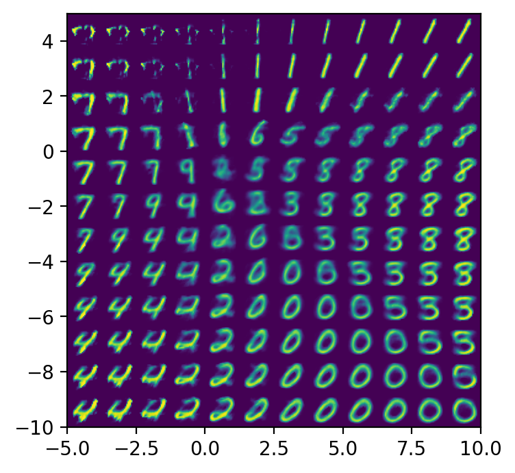
Figure 5 – MNIST reconstruction samples from latent space

This degradation is not merely a failure of capacity, but a fundamental architectural flaw when dealing with high-dimensional spatial data:

1. Loss of Spatial Locality: By flattening a 2D image into a 1D vector, the MLP destroys the local grid structure. It treats two adjacent pixels with the exact same mathematical independence as two pixels on opposite corners of the image.
2. Lack of Translation Invariance: If a feature (like a curved edge) appears in the top-left of an image during training, an MLP must learn a completely separate set of weights to recognize that exact same edge if it appears in the bottom-right.
3. Parameter Inefficiency: Fully connected layers require a massive number of parameters. Scaling an MLP to handle high-resolution images (e.g., $1024 \times 1024 \times 3$) becomes computationally intractable and highly prone to overfitting.

To effectively reconstruct and generate high-fidelity spatial data, the architecture must natively respect local correlations—a requirement that leads us directly to the Convolutional Autoencoder.

4. The Convolutional Neural Network (CNN) Autoencoder

As established in the previous section, treating high-dimensional spatial data (like images) as flattened one-dimensional vectors strips away critical structural context. The Multilayer Perceptron is fundamentally agnostic to spatial locality. To build an autoencoder capable of capturing the rich, hierarchical structure of visual data, we must embed a strong inductive bias into the architecture. The Convolutional Neural Network (CNN) Autoencoder achieves this by leveraging local receptive fields, shared weights, and spatial pooling.

4.1. Spatial Coherence and the Convolutional Inductive Bias

Natural images contain profound local correlations; adjacent pixels are highly likely to share similar properties and belong to the same structural features (e.g., edges, textures). A CNN autoencoder respects this spatial coherence through the convolution operation.

Instead of learning a unique, dense weight for every pixel combination, a convolutional encoder sweeps learned filters (kernels) across the input. This provides two critical theoretical advantages:

1. Parameter Efficiency: The weights of a kernel are shared across the entire spatial domain, drastically reducing the parameter count and mitigating the risk of overfitting on high-resolution data.
2. Translation Invariance: A feature learned in one region of the image can be seamlessly recognized in another. If the encoder learns a Gabor-like filter to detect a vertical edge in the top-left corner, that exact same filter will successfully encode a vertical edge in the bottom-right.

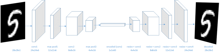
Figure 6 – CNN autoencoder architecture showing spatial down-sampling through convolutions and up-sampling through transposed convolutions, converging at a dense bottleneck [4].

4.2. Downsampling and Upsampling Mechanics

A CNN autoencoder replaces dense compression with a geometric reduction of spatial dimensions accompanied by an expansion in channel depth.

• The Convolutional Encoder (Downsampling): As the input tensor passes through successive convolutional layers, we typically apply a stride of $s > 1$ (or use pooling layers, though strided convolutions are generally preferred in modern architectures to allow the network to learn its own spatial downsampling). For a spatial dimension of $W_{in}$, a convolutional layer with a kernel size $K$, padding $P$, and stride $S$ reduces the output dimension to: $W_{out} = \lfloor \frac{W_{in} + 2P – K}{S} \rfloor + 1$. This process increases the receptive field of the deeper neurons, allowing the network to encode highly abstract, global features into the latent space while squashing the spatial grid.
• The Convolutional Decoder (Upsampling): To reconstruct the original input, the decoder must invert this spatial compression. This is mathematically achieved using Transposed Convolutions (sometimes inaccurately referred to as “deconvolutions”). A transposed convolution broadcasts an input activation across a spatial neighborhood weighted by the kernel, effectively expanding the feature map. Careful selection of the output_padding parameter is often required to resolve dimensional ambiguities that arise during strided downsampling, ensuring the reconstructed tensor perfectly matches the original image resolution.

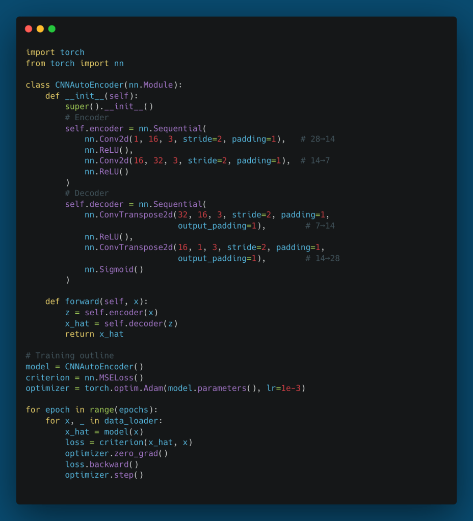
4.3. PyTorch Implementation

The following implementation demonstrates a robust CNN autoencoder designed for single-channel images like MNIST. Notice how the encoder transforms the spatial tensor into a true vector bottleneck to force holistic representation learning, before reshaping it for the spatial decoder.

4.4. Comparative Analysis: MLP vs. CNN Autoencoders

When comparing the empirical results of CNN autoencoders against their MLP counterparts on visual data, the theoretical advantages of convolutional architectures translate into stark performance differences:

The CNN autoencoder thus forms the essential bridge between simple reconstructive networks and modern, high-fidelity computer vision systems. By successfully mapping high-dimensional spatial data into reliable, dense latent codes, these networks unlock powerful downstream applications. In the next section, we will explore how this reconstructive capacity is practically deployed to solve unsupervised problems, most notably in the domain of anomaly detection.

5. Practical Applications: Anomaly Detection and Beyond

While autoencoders are fundamentally designed for representation learning, their unique ability to learn the intrinsic structure of a dataset without labels makes them incredibly powerful for applied machine learning. One of the most ubiquitous and commercially valuable applications of this architecture is unsupervised anomaly detection. By leveraging the reconstruction error as a measurable proxy for “normality,” we can identify out-of-distribution events in complex, high-dimensional spaces where traditional rule-based logic fails.

5.1. The Principle of Anomaly Detection

The mathematical intuition behind autoencoder-based anomaly detection relies on the geometry of the latent space.

During the training phase, the autoencoder is exposed exclusively to “normal” or baseline data. Consequently, the encoder learns to map only the manifold of this normal distribution, and the decoder learns to project from this specific subspace back to the original dimensions. The network allocates its limited parameter capacity entirely to minimizing the reconstruction loss of typical structural patterns.

During inference, when the network encounters an anomalous input $\mathbf{x}_{\text{anom}}$(e.g., a defective part, a fraudulent transaction, or a network intrusion), the encoder is forced to project this unseen pattern onto the nearest point of the “normal” latent manifold. Because the anomaly lacks the structural correlations the network was optimized for, the decoder will reconstruct it poorly, yielding a high reconstruction error.

The anomaly detection pipeline is formalized as follows:

1. Compute Reconstruction Error: For a new sample $\mathbf{x},$compute $E(\mathbf{x}) = |\mathbf{x} – f_{\text{dec}}(f_{\text{enc}}(\mathbf{x}))|_2^2$.
2. Establish a Threshold: Define a scalar threshold $\tau$. This is typically derived statistically from the validation set of normal data (e.g., the 95th or 99th percentile of baseline reconstruction errors).
3. Classification: If $E(\mathbf{x}) > \tau$, flag the sample as anomalous.

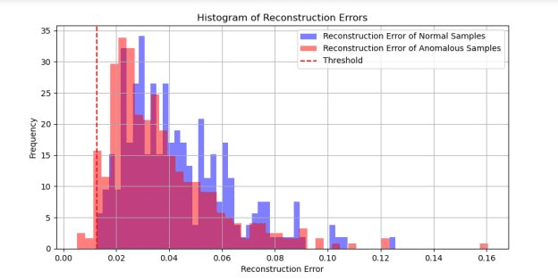
Figure 8 – Anomaly detection thresholding concept. A histogram showing the distribution of reconstruction errors for normal data versus anomalous data, illustrating the separability provided by the threshold [5].

5.2. Cross-Domain Applications

This reconstructive approach to outlier detection is highly adaptable and has been deployed across numerous technical domains:

• Industrial Robotics and Predictive Maintenance: Modern robotic arms and CNC machines generate continuous streams of multivariate sensor data (e.g., joint torques, vibrations, acoustic emissions). By training an MLP or 1D-CNN autoencoder on data from healthy operational cycles, engineers can monitor the real-time reconstruction loss. A gradual upward trend in $E(\mathbf{x})$ often indicates mechanical wear or impending bearing failure long before it causes a catastrophic shutdown.
• Automated Visual Inspection: In semiconductor manufacturing or textile production, labeling every possible defect type (scratches, misalignments, impurities) is impossible. A CNN autoencoder trained solely on flawless components will fail to reconstruct a scratch on a silicon wafer. By examining the pixel-wise difference between the input image and the reconstruction ($|\mathbf{x} – \hat{\mathbf{x}}|$), the system can instantly generate a heatmap localizing the exact position of the defect.
• Cybersecurity and Intrusion Detection: Network traffic patterns can be encoded into feature vectors (e.g., packet sizes, sequence timing, protocol types). Sequence-based autoencoders (using 1D Convolutions or LSTMs) trained on routine network traffic will output massive reconstruction spikes when encountering the novel payload structures or timing anomalies characteristic of zero-day exploits or DDoS attacks.

5.3. Expanding Utility: Denoising and Pretraining

Beyond anomaly detection, the autoencoder framework serves as a versatile utility belt for data scientists:

• Denoising Autoencoders (DAE): DAE intentionally corrupts the input data with stochastic noise (e.g., $\tilde{\mathbf{x}} = \mathbf{x} + \mathcal{N}(0, \sigma^2)$ or random dropout) but calculates the loss against the clean original target. This severs the identity mapping entirely, forcing the network to learn robust, invariant features that capture the true data-generating distribution rather than local noise.
• Dimensionality Reduction: The bottleneck layer provides a powerful non-linear alternative to PCA. Extracting the latent vectors yields dense, informative embeddings that can be fed into traditional clustering algorithms (like DBSCAN) or projected into 2D/3D spaces using algorithms like t-SNE and UMAP for data visualization.
• Unsupervised Pretraining: In domains where unlabeled data is abundant but labeled data is scarce (e.g., medical imaging), an autoencoder can be trained on the massive unlabeled corpus. The decoder is then discarded, and the pre-trained encoder weights are transferred to initialize a supervised classification network. This provides a massive head start on feature extraction, leading to faster convergence and higher accuracy on the limited labeled dataset.

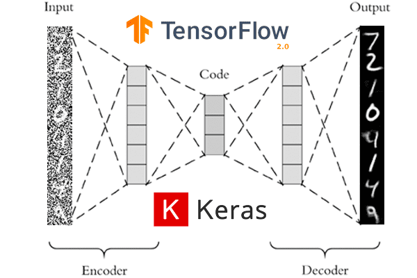
Figure 9 – Examples of the Denoising Autoencoder process. The network successfully removes injected Gaussian noise, recovering the underlying signal structure [6].

6. The Generative Extension: Variational Autoencoders (VAE)

The standard autoencoder is a powerful tool for compression and feature extraction, but it harbors a critical limitation: it is not a generative model. Because the standard autoencoder is trained deterministically to minimize reconstruction error, its latent space is highly irregular and discontinuous. If you sample an arbitrary point $\mathbf{z}$ from the latent space of an MLP or CNN autoencoder, the decoder will likely output meaningless noise.

To transition from a reconstructive model to a true generative model, we must enforce a continuous, densely packed probabilistic structure on the latent space. This is the foundational breakthrough of the Variational Autoencoder (VAE).

6.1. From Deterministic Encoding to Probabilistic Inference

In a classical autoencoder, the encoder maps an input $\mathbf{x}$ to a single, discrete latent vector $\mathbf{z}$. In a VAE, the encoder maps the input to a probability distribution over the latent space.

Specifically, the encoder $q_\phi(\mathbf{z}|\mathbf{x})$ outputs the parameters of a multivariate Gaussian distribution: a mean vector $\boldsymbol{\mu}$ and a variance vector $\boldsymbol{\sigma}^2$.

During the forward pass, the latent representation $\mathbf{z}$ is stochastically sampled from this distribution:

This probabilistic mapping ensures that similar inputs are encoded into overlapping topological regions, creating a smooth, continuous manifold where every local point corresponds to a valid, sensible reconstruction.

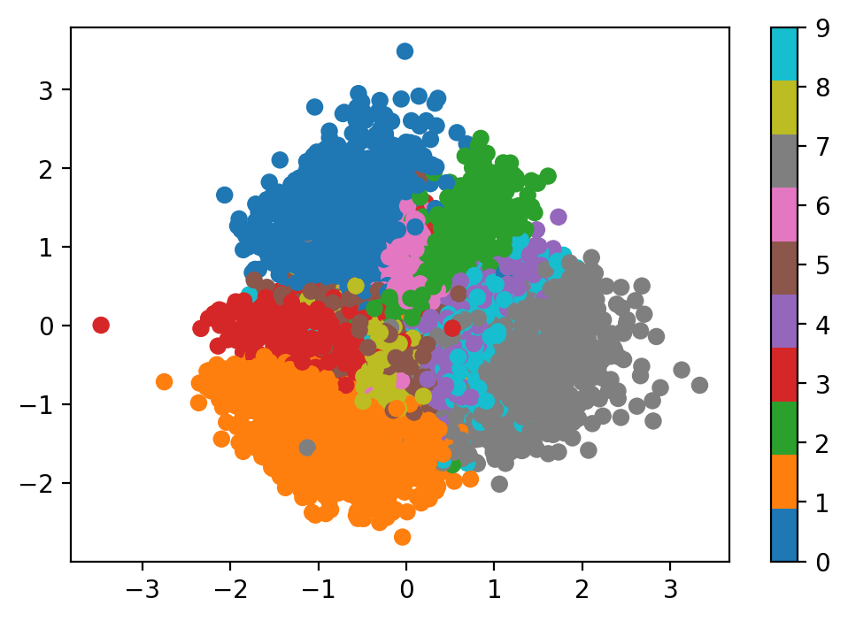
Figure 10 – Comparison of latent spaces. The standard autoencoder creates isolated points, while the VAE creates overlapping Gaussian spheres, ensuring a continuous generative manifold [7].

6.2. The Reparameterization Trick

A fundamental engineering challenge arises when introducing stochastic sampling into a neural network: you cannot backpropagate gradients through a random sampling operation. The sampling step blocks the deterministic chain rule required to update the encoder’s weights $\phi$.

The reparameterization trick elegantly resolves this by mathematically decoupling the randomness from the learned parameters. Instead of sampling $\mathbf{z}$ directly from the parameterized distribution, we sample a noise variable $\boldsymbol{\epsilon}$ from a standard unit Gaussian prior, $\mathcal{N}(0, \mathbf{I})$, and deterministically scale and shift it:

By routing the stochasticity into the independent auxiliary variable $\boldsymbol{\epsilon}$, the operations acting on $\boldsymbol{\mu}$ and $\boldsymbol{\sigma}$ become standard differentiable nodes in the computational graph.

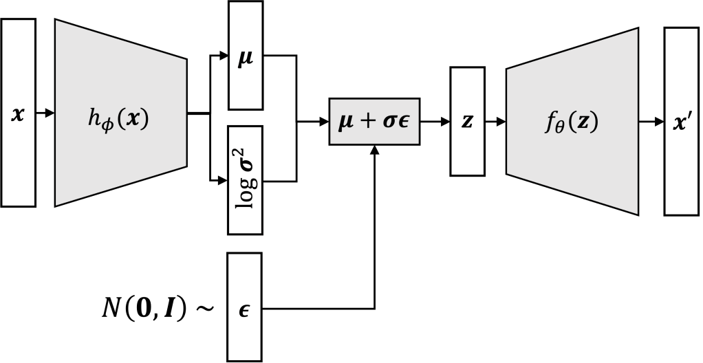
Figure 11 – The Reparameterization Trick. A computational graph showing how the stochastic node is sidestepped to allow uninterrupted gradient flow back to the encoder [2].

6.3. The Evidence Lower Bound (ELBO)

Training a VAE requires optimizing a dual-objective loss function. We want to maximize the likelihood of the data while ensuring the learned latent distributions closely resemble a chosen prior (typically a standard normal distribution). We achieve this by maximizing the Evidence Lower Bound (ELBO), which translates to minimizing the following loss function:

This equation consists of two opposing forces:

1. The Reconstruction Loss (first term): Measures how well the decoder $p_\theta(\mathbf{x}|\mathbf{z})$ reconstructs the input from the sampled latent vector. This is typically implemented as Mean Squared Error (MSE) or Binary Cross-Entropy (BCE).
2. The Kullback-Leibler (KL) Divergence (second term): Acts as a powerful regularizer. It measures the statistical distance between the encoder’s predicted distribution $q_\phi(\mathbf{z}|\mathbf{x})$ and the standard normal prior $p(\mathbf{z}) = \mathcal{N}(0, \mathbf{I})$. It mathematically forces the latent distributions to pack closely around the origin, preventing the network from “cheating” by placing distributions infinitely far apart to avoid overlap.

For a multivariate Gaussian with diagonal covariance, the KL divergence term has a closed-form analytical solution:

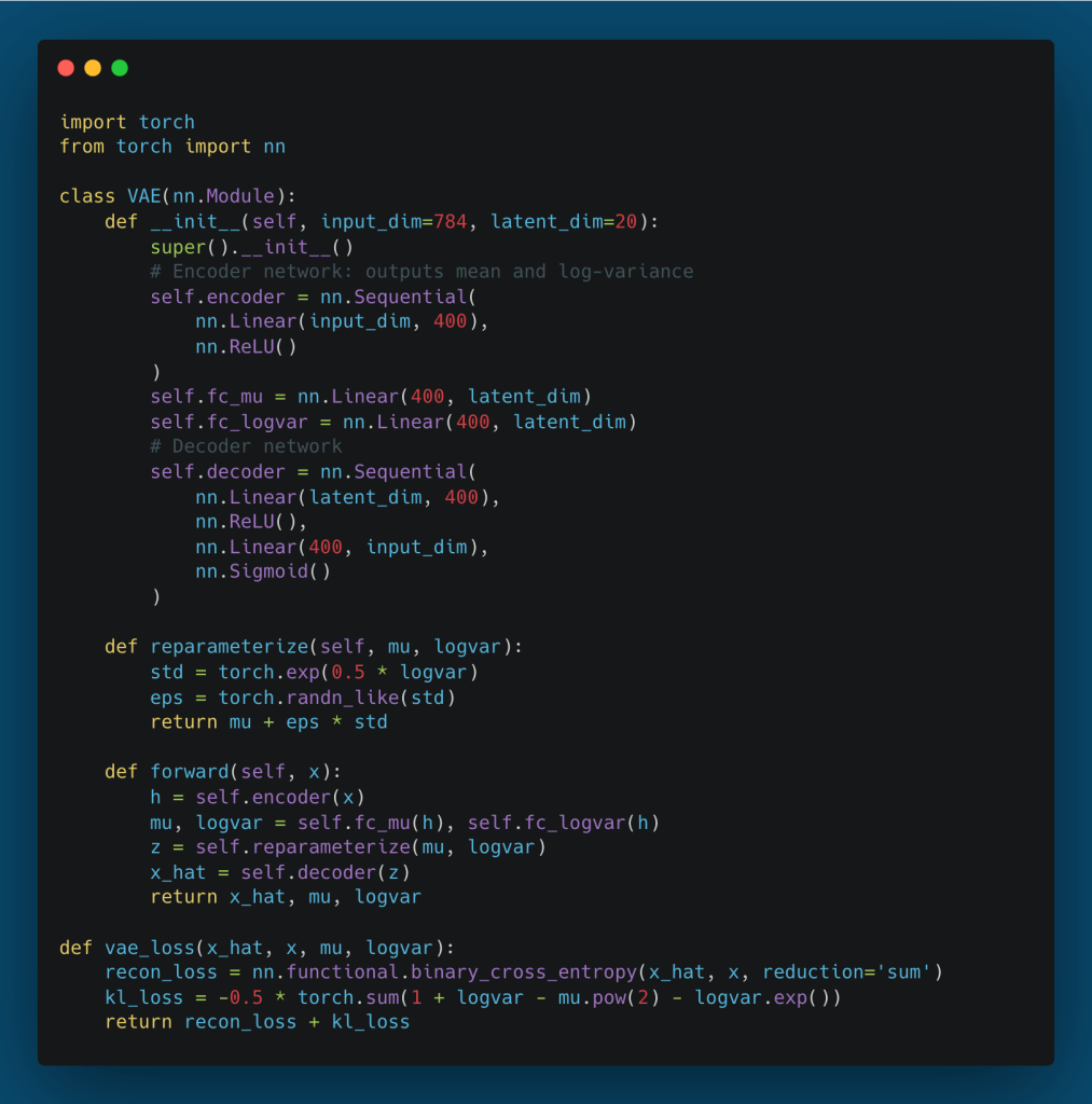
6.4. PyTorch Implementation

In practice, for numerical stability, the encoder is designed to output the log-variance ($\log \sigma^2$) rather than the variance directly.

6.5. Generative Sampling and Latent Space Interpolation

Once the VAE is trained, the encoder is completely discarded for generation tasks. To synthesize entirely novel data, we simply sample a vector $\mathbf{z}$ from the prior $\mathcal{N}(0, \mathbf{I})$ and pass it through the decoder.

Furthermore, because the KL divergence forces the space to be dense and continuous, we can perform latent space interpolation. By taking the latent vectors of two distinct real images ($\mathbf{z}_A$ and $\mathbf{z}_B$) and calculating the linear sequence between them ($\mathbf{z}_t = (1-t)\mathbf{z}_A + t\mathbf{z}_B$), the decoder will generate a sequence of images that smoothly morphs from the first image to the second, representing structurally valid, intermediate semantic concepts.

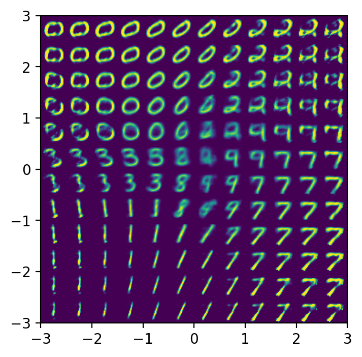
Figure 12 – Latent interpolation between MNIST digits, demonstrating how the model learns smooth semantic transitions (e.g., a “3” morphing cleanly into an “8”) rather than abrupt, noisy pixel shifts.

6.6. Legacy in Modern Generative AI

The Variational Autoencoder was a paradigm shift. Its probabilistic formulation of latent spaces served as the conceptual and architectural foundation for the current era of generative AI:

• $\beta$-VAEs: Introduced a scaling factor to the KL divergence term, allowing researchers to force the network to learn highly disentangled representations (e.g., separating object color from object orientation into distinct latent dimensions).
• VQ-VAEs (Vector Quantized VAEs): Replaced the continuous Gaussian latent space with a discrete codebook. This solved the “blurriness” issue often associated with standard VAEs and became the foundational architecture for generating high-fidelity audio and images.
• Latent Diffusion Models: Systems like Stable Diffusion rely heavily on VAEs. Instead of running the expensive diffusion denoising process in raw, high-resolution pixel space, these models compress the image using a VAE encoder, perform diffusion strictly within the low-dimensional latent space, and then decode the result back to high resolution.

7. Conclusion

Autoencoders represent a masterclass in the power of architectural constraints. By simply forcing a neural network to compress and reconstruct its own input, we transition from relying on expensive, human-annotated labels to unlocking the intrinsic, self-supervised structure of the data itself.

Throughout this post, we have traced the evolution of this architecture:

• We began with the mathematical foundations of the encoder-decoder mapping and the probabilistic assumptions underlying standard reconstruction losses.
• We explored the MLP Autoencoder, understanding its utility for structured data but acknowledging its severe limitations regarding spatial locality and parameter efficiency.
• We solved those spatial limitations with the CNN Autoencoder, leveraging the inductive biases of convolutional filters to achieve high-fidelity image compression and feature extraction.
• We examined the immense practical value of these deterministic networks, particularly in unsupervised anomaly detection, where reconstruction error serves as a reliable boundary for normality across industrial, cybersecurity, and medical domains.
• Finally, we broke the deterministic barrier with the Variational Autoencoder (VAE). By introducing probabilistic inference, the reparameterization trick, and the ELBO objective, we transformed a simple reconstructive tool into a continuous, interpolatable generative model—laying the conceptual groundwork for the modern era of Generative AI.

Whether you are building a predictive maintenance pipeline to detect manufacturing anomalies, or studying the latent diffusion models that power today’s state-of-the-art image synthesis, the autoencoder remains an indispensable architectural pillar in the deep learning repertoire.

Hands-On Exploration: Interactive Autoencoder Framework

If you want to move beyond the theory and experiment with these architectures firsthand, I have built a modular, Interactive Autoencoder Framework available on my GitHub:

https://github.com/turhancan97/simple-autoencoder-demo

This repository provides a complete, YAML-configurable PyTorch pipeline to train and visualize MLP, CNN, and VAE models on datasets like MNIST. Its standout feature is the real-time demo.py application, which generates a visual 2D mapping of the trained bottleneck. By simply clicking and dragging your mouse across the latent space clusters, you can watch the decoder continuously generate and morph reconstructions in real-time. It is an excellent practical tool for observing the structural differences between the deterministic latent space of a standard MLP and the smooth, continuous generative manifold of a VAE.

Reference

1. Dense in. Stack Overflow. Stack Overflow. Published 2019. Accessed October 30, 2025. https://stackoverflow.com/questions/55233114/how-to-create-autoencoder-using-dropout-in-dense-layers-using-keras
2. ‌Matthew Bernstein. Matthew N. Bernstein. Published March 14, 2023. Accessed October 30, 2025. https://mbernste.github.io/posts/vae/
3. ‌rvislaywade. Visualizing MNIST using a Variational Autoencoder. Kaggle.com. Published March 8, 2018. Accessed October 30, 2025. https://www.kaggle.com/code/rvislaywade/visualizing-mnist-using-a-variational-autoencoder
4. ‌Deep Discriminative Latent Space for Clustering. ResearchGate. Published online 2018. doi:https://doi.org/10.48550//arXiv.1805.10795
5. AutoEncoder Convolutional Neural Network for Pneumonia Detection. (2024). ResearchGate. https://doi.org/10.48550//arXiv.2409.02142
6. ‌Rosebrock, A. (2020, February 24). Denoising autoencoders with Keras, TensorFlow, and Deep Learning – PyImageSearch. PyImageSearch. https://pyimagesearch.com/2020/02/24/denoising-autoencoders-with-keras-tensorflow-and-deep-learning/
7. ‌Van, A. (2020, May 14). Alexander Van de Kleut. Alexander van de Kleut. https://avandekleut.github.io/vae/

Merhaba sevgili okurlar! Serimizin önceki bölümünde palindrome kelimeleri Java dilini kullanarak nasıl kontrol edeceğimizi öğrenmiştik. Bugün ise sizlerle birlikte Sayısal Loto için küçük çaplı bir sayı üreteci yapacağız. Bu bölümde, Python dilini kullanacağız. Hazırsanız, başlayalım!

Oyunun Amacı

Sayısal Loto, çeşitli ülkelerde popüler olan bir şans oyunudur. Oyunda, belirli bir aralıktaki sayılardan belirli bir miktarını doğru tahmin etmek gerekiyor. Bizim amacımız ise Python dilini kullanarak tekrarlamadan 6 adet sayı üreten bir Sayısal Loto uygulaması yapmak.

Algoritmanın Çalışma Prensibi

Algoritma, temel olarak iki adet döngü ile çalışır. İlk döngü, rasgele bir sayı üretir ve bu sayı, sayıların bulunduğu diziye atanır. İkinci döngü ise, bu sayının daha önce dizide var olup olmadığını kontrol eder. Eğer sayı dizi içinde yoksa, bu sayı diziye eklenir. Eğer sayı dizi içinde varsa, yeni bir sayı üretilir ve bu işlem sayı dizi içinde yok olana kadar tekrar edilir.

Python’da Sayısal Loto Uygulaması

Python dilini kullanarak tekrarsız 6 adet sayı üreten bir Sayısal Loto uygulaması yapalım. İşte kodumuz:

import random

numbers = []
while len(numbers) < 6:
    number = random.randint(1, 49)
    if number not in numbers:
        numbers.append(number)

print(sorted(numbers))

Bu kodda, önce numbers adında boş bir liste oluşturduk. Daha sonra, while döngüsü içinde, 6 adet sayı elde edene kadar rasgele sayı üretiyoruz. Eğer üretilen sayı numbers listesinde yoksa, bu sayıyı listeye ekliyoruz. Son olarak, üretilen sayıları küçükten büyüğe sıralayarak ekrana yazdırıyoruz.

Program çıktı örnekleri:

>> [10, 12, 13, 23, 41, 47]
>> [6, 12, 16, 17, 19, 21]
>> [8, 14, 18, 19, 33, 37]

Algoritmanın Zaman ve Hafıza Karmaşıklığı

Bu algoritmanın zaman karmaşıklığı, en kötü durumda O(n²) ve ortalama durumda O(n log n) olacaktır. Çünkü her bir yeni sayının listeye eklenmeden önce listeye ait olup olmadığını kontrol etmek için tüm liste taranmaktadır.

Hafıza karmaşıklığı ise O(n)’dir. Çünkü her bir yeni sayı listeye eklenirken, hafızada yeni bir yer ayrılıyor. Bu durumda n, listemizdeki öğe sayısına denk gelmektedir.

Sonuç

Bu yazıda, Sayısal Loto için küçük çaplı bir sayı üreteci oluşturmanın temellerini öğrendik. Python kullanarak tekrarlamadan 6 adet sayı üreten bir programı nasıl oluşturacağımızı gördük. Bu örnek, tekrar etmeyen sayıların nasıl üretilebileceği ve bir dizi içerisinde nasıl saklanacağı konularında da bize yol göstermiştir.

Bu yazıyla birlikte bu seriyi sonlandırıyoruz. Algoritma ve Programlama Dünyası serisi adı altında, Üniversitede alabileceğiniz programlamaya giriş derslerinde işleyebileceğiniz hemen hemen her konuya baktık. Umarım bu seriden keyif almışsınızdır. Bundan sonraki yazılarda mutlaka yeni projeler ve uygulamalar yapacağız ancak bunlar muhtemelen herhangi bir yazı dizisinde yer almayacak. Kendinize iyi bakın, happy coding!

Eğer bu yazıyı beğendiyseniz aşağıdaki alkışa istediğiniz kadar tıklayarak yazılarıma destek olabilirsiniz :)

Herhangi bir sorunuz olursa veya benimle iletişim kurmak isterseniz, tüm sosyal medya hesaplarım aşağıdaki linkte yer alıyor.

Turhan Can Kargin | Home

Ayrıca diğer blog yazılarımı aşağıda yer alan websitem üzerinden takip edebilirsiniz.

Turhan Can Kargın

Bir sonraki yazıda görüşmek üzere!

Herkese merhabalar! Önceki yazılarımızda bir dizi sıralama algoritmasını Python ve C++ gibi dillerle uygulamayı gördük. Son yazımızda ise basit bir tahmin oyunu yapmıştık. Bu sefer, çeşitli alanlarda kullanılan bir başka önemli algoritma türüne odaklanacağız: Palindrom kontrolü. Bu uygulamayı Java dilinde gerçekleştireceğiz.

Palindrome Nedir?

Palindrom bir kelime, cümle veya sayı dizisinin ileriye veya geriye doğru aynı şekilde okunabilmesidir. Örneğin ‘madam’, ‘racecar’ veya ‘121’ gibi. Palindromlar, algoritma ve veri yapıları derslerinde sıkça kullanılan bir konsepttir. Bunun yanında, genetik dizilerin incelenmesi ve bazı arama algoritmaları gibi birçok gerçek dünya uygulaması da bulunmaktadır.

Palindrome Kontrol Algoritması

Palindrome kontrol algoritması, bir kelimenin veya cümlenin palindrom olup olmadığını kontrol eder. Bu, genellikle bir kelimenin ilk ve son karakterlerini karşılaştırarak ve daha sonra kelimenin içine doğru ilerleyerek yapılır.

Pseudocode (Sözde Kod)

ALGORITMA IsPalindrome
GİRDİ: String str
ÇIKTI: Boolean

BAŞLA
  SET start TO 0
  SET end TO length of str - 1
  
  WHILE start < end DO
    IF str[start] != str[end] THEN
      RETURN false
    END IF
    
    INCREMENT start
    DECREMENT end
  END WHILE
  
  RETURN true
BİTİR

Java’da Palindrome Kontrol Uygulaması

public class Main {
    public static boolean isPalindrome(String str) {
        int start = 0, end = str.length() - 1;
  
        while (start < end) {
            if (str.charAt(start) != str.charAt(end))
                return false;
  
            start++;
            end--;
        }
  
        return true;
    }

    public static void main(String[] args) {
        String str1 = "madam";
        String str2 = "hello";

        System.out.println("Is '" + str1 + "' a palindrome? " + isPalindrome(str1));
        System.out.println("Is '" + str2 + "' a palindrome? " + isPalindrome(str2));
    }
}

Bu kod, belirtilen stringin palindrom olup olmadığını kontrol eder ve sonucu ekrana basar.

Çıktılar:

Is 'madam' a palindrome? true
Is 'hello' a palindrome? false

Bu çıktılar, “madam” kelimesinin bir palindrom olduğunu (ilk ve son harfler aynı ve bu durum kelimenin tümünde geçerli) ve “hello” kelimesinin bir palindrom olmadığını (ilk ve son harfler farklı) gösterir.

Algoritmanın Zaman Karmaşıklığı

Palindrome kontrol algoritmasının zaman karmaşıklığı genellikle O(n) olarak kabul edilir, çünkü stringin her karakteri en fazla bir kez kontrol edilir.

Sonuç

Java’da palindrome kontrol algoritması, genel amaçlı ve genellikle string işleme problemlerini çözmek için kullanılır. Hem pratikte hem de kodlama mülakatlarında sıkça karşılaşılan bir konudur. Palindrom kontrol algoritması, bir algoritmanın basitliği ile onun etkinliği arasındaki dengeyi güzel bir şekilde gösterir.

Eğer bu yazıyı beğendiyseniz aşağıdaki alkışa istediğiniz kadar tıklayarak yazılarıma destek olabilirsiniz :)

Herhangi bir sorunuz olursa veya benimle iletişim kurmak isterseniz, tüm sosyal medya hesaplarım aşağıdaki linkte yer alıyor.

Turhan Can Kargin | Home

Ayrıca diğer blog yazılarımı aşağıda yer alan websitem üzerinden takip edebilirsiniz.

Turhan Can Kargın

Bir sonraki yazıda görüşmek üzere!

<hr><p>Algoritma ve Programlama Dünyası — Uygulama 8 (Palindrome Kelimeler) was originally published in Kodcular on Medium, where people are continuing the conversation by highlighting and responding to this story.</p>

Merhaba sevgili okuyucular! Algoritmaların sadece karmaşık problemleri çözmek için değil, aynı zamanda eğlenceli ve etkileşimli oyunlar oluşturmak için de kullanılabileceğini biliyor muydunuz? Serimizin önceki bölümlerinde, birçok popüler sıralama algoritması hakkında konuştuk. Bu yazıda ise biraz eğlenelim ve basit bir tahmin oyunu yapalım! Bu oyunu C++ dilinde gerçekleştireceğiz!

Oyunun Amacı

Oyunumuzun temel amacı, kullanıcının belirli bir sayıyı tahmin etmesidir. Program, her başlangıçta 1 ile 50 arasında rastgele bir sayı üretir. Kullanıcıya bu sayıyı tahmin etmek için 5 hakkı vardır. Kullanıcının tahmin ettiği sayı üretilen sayıdan daha büyükse, “Sayıyı Küçült” mesajı gösterilir. Tahmin edilen sayı daha küçükse, “Sayıyı Büyüt” mesajı gösterilir. Kullanıcı sayıyı tahmin ettiğinde, “Tebrikler” mesajı gösterilir ve oyun sona erer. Ancak, kullanıcı tüm haklarını kullanırsa ve hala sayıyı tahmin edemezse, “Kaybettin” mesajı gösterilir ve oyun sona erer.

Oyunun Algoritması

Oyunumuzun algoritmasını Pseudocode (Sözde Kod) ile aşağıda belirtelim:

BAŞLA
  rastgele_sayi = 1 ile 50 arasında rastgele sayı üret
  haklar = 5
  
  DÖNGÜ haklar > 0 olarak:
    tahmin = kullanıcıdan sayı al
    
    EĞER tahmin > rastgele_sayi ise:
      yazdır("Sayıyı Küçült")
    YOKSA EĞER tahmin < rastgele_sayi ise:
      yazdır("Sayıyı Büyüt")
    YOKSA:
      yazdır("Tebrikler")
      ÇIKIŞ
    haklar = haklar - 1

  yazdır("Kaybettin")
BİTİR

C++’da Tahmin Oyunu Uygulaması

C++’da Tahmin Oyunu’nun uygulamasına geçmeden önce, C++’nın rastgele sayı üretme özelliklerine aşina olmamız gerekiyor. C++’da rastgele sayı üretmek için <random> kütüphanesini kullanırız. Ayrıca girdi/alma işlemleri için <iostream> kütüphanesini kullanacağız. Bu kütüphanelerin yardımıyla, oyunumuzun uygulamasını gerçekleştirebiliriz.

C++ dilindeki kodumuzu aşağıda bulabilirsiniz. (Kodun nasıl çalıştığını anlamak için her bir satırı dikkatlice okuyunuz.)

#include <iostream>
#include <random>

int main() {
  std::random_device rd;
  std::mt19937 gen(rd());
  std::uniform_int_distribution<> distr(1, 50);

  int rastgele_sayi = distr(gen);
  int haklar = 5;
  int tahmin;

  while (haklar > 0) {
    std::cout << "Bir sayı tahmin edin: ";
    std::cin >> tahmin;

    if (tahmin > rastgele_sayi) {
      std::cout << "Sayıyı Küçült!\n";
    } else if (tahmin < rastgele_sayi) {
      std::cout << "Sayıyı Büyüt!\n";
    } else {
      std::cout << "Tebrikler, sayıyı doğru tahmin ettiniz!\n";
      return 0;
    }

    haklar--;
  }

  std::cout << "Üzgünüm, tüm haklarınızı kullandınız. Kaybettiniz!\n";

  return 0;
}

Örnek çıktılar aşağıda verilmiştir:

Bir sayı tahmin edin: 25
Sayıyı Küçült!
Bir sayı tahmin edin: 10
Sayıyı Büyüt!
Bir sayı tahmin edin: 17
Sayıyı Büyüt!
Bir sayı tahmin edin: 21
Sayıyı Küçült!
Bir sayı tahmin edin: 19
Tebrikler, sayıyı doğru tahmin ettiniz!

Bir sayı tahmin edin: 25
Sayıyı Küçült!
Bir sayı tahmin edin: 15
Sayıyı Küçült!
Bir sayı tahmin edin: 10
Sayıyı Küçült!
Bir sayı tahmin edin: 4
Sayıyı Büyüt!
Bir sayı tahmin edin: 7
Sayıyı Büyüt!
Üzgünüm, tüm haklarınızı kullandınız. Kaybettiniz!

Algoritmanın Zaman ve Hafıza Karmaşıklığı

Oyunumuzun zaman ve hafıza karmaşıklığına gelirsek, kullanıcıdan bir sayı alıp karşılaştırma işlemini 5 kez tekrarlıyoruz. Bu yüzden zaman karmaşıklığımız O(1), yani sabittir. Hafıza karmaşıklığı da O(1) olarak kabul edilebilir, çünkü sabit sayıda değişkenimiz var ve bu değişkenlerin sayısı girdinin büyüklüğüne bağlı değildir.

Bu oyun, algoritmaları daha iyi anlamanıza ve C++ dilini daha etkin bir şekilde kullanmanıza yardımcı olacaktır. Bol pratik yapın ve eğlenin!

Umarım bu yazı, algoritmalar ve programlama hakkında bilginizi geliştirmenize yardımcı olmuştur. Sorularınız varsa, yorum bırakmayı unutmayın. Bir sonraki yazıda görüşmek üzere!

Eğer bu yazıyı beğendiyseniz aşağıdaki alkışa istediğiniz kadar tıklayarak yazılarıma destek olabilirsiniz :)

Herhangi bir sorunuz olursa veya benimle iletişim kurmak isterseniz, tüm sosyal medya hesaplarım aşağıdaki linkte yer alıyor.

Turhan Can Kargin | Home

Ayrıca diğer blog yazılarımı aşağıda yer alan websitem üzerinden takip edebilirsiniz.

Turhan Can Kargın

Bir sonraki yazıda görüşmek üzere!

<hr><p>Algoritma ve Programlama Dünyası — Uygulama 7 (Tahmin Oyunu) was originally published in Kodcular on Medium, where people are continuing the conversation by highlighting and responding to this story.</p>

The Current Landscape of AI

Artificial Narrow Intelligence (ANI): A World of Specialized Wizards

Today’s AI landscape is dominated by Artificial Narrow Intelligence (ANI), systems designed to perform specific tasks with a level of proficiency that can sometimes surpass human capabilities. These specialized wizards are the workhorses behind some of the most impactful technological innovations of our era. From the voice assistants in our homes to the sophisticated algorithms guiding self-driving cars, ANI has permeated various aspects of our daily lives, often invisibly and seamlessly.

ANI applications are diverse, covering a range of domains such as web search engines that sift through the vast expanse of the internet to deliver precise information, smart agriculture systems optimizing crop yields, and automated manufacturing processes revolutionizing factories. The success of ANI lies in its focus: by concentrating on narrowly defined tasks, these AI systems achieve incredible accuracy and efficiency, creating substantial value across industries.

Progress and Misconceptions

The rapid progress in ANI over the last decade has been nothing short of remarkable. Breakthroughs in machine learning, particularly deep learning, have enabled significant advancements in pattern recognition, natural language processing, and predictive analytics. This progress, however, has led to a widespread misconception about the state of AI as a whole. The leap from mastering specific tasks to achieving a general, human-like intelligence is not merely a matter of scale but a fundamental shift in capability.

While ANI focuses on doing one thing exceptionally well, the dream of AGI is to create systems that can understand, learn, and apply knowledge across a broad range of tasks, adapting to new challenges with the flexibility and ingenuity of a human mind. Despite the excitement and optimism generated by advancements in ANI, the truth remains that we are still far from realizing AGI. The distinction between these two concepts is crucial for setting realistic expectations about the future of AI and guiding research efforts towards meaningful breakthroughs.

As we navigate the current landscape of AI, it’s essential to recognize the achievements and limitations of ANI while keeping the long-term goal of AGI in perspective. This understanding not only frames our expectations but also highlights the vast potential and challenges that lie ahead on the path to achieving artificial general intelligence.

The AGI Dream and Its Challenges

The dream of Artificial General Intelligence (AGI) stretches far beyond the capabilities of today’s AI, envisioning a future where machines can rival human intellect across all aspects of learning, reasoning, and creativity. This vision for AGI is not just about creating technology that can perform tasks with human-like efficiency; it’s about forging an entity that understands and interacts with the world in a way indistinguishable from humans. However, the path to AGI is fraught with unprecedented challenges, both technical and philosophical, that extend the timeline of its realization into an uncertain future.

The Complexity of Human Intelligence

One of the foremost challenges in achieving AGI is the sheer complexity of human intelligence. Our cognitive abilities arise from intricate interactions within networks of billions of neurons, shaped by millennia of evolutionary pressures. Replicating this level of complexity in a machine requires not just an understanding of how individual neurons function but how the emergent properties of consciousness and intelligence arise from the vast networks of these biological units. The endeavor to create AGI thus involves deciphering the deepest mysteries of the human mind, a task that intersects with the realms of neuroscience, psychology, and even philosophy.

The Hype and Its Consequences

Amidst the significant progress in AI, particularly in domains governed by ANI, a narrative suggesting that AGI is just around the corner has gained traction. This hype, often amplified by sensational media coverage and speculative futurism, obscures the reality of the scientific and engineering challenges ahead. While optimism fuels progress, unrealistic expectations can lead to disappointment, eroding public trust and potentially diverting attention and resources from the foundational research required to advance towards AGI.

Ethical Considerations

As we ponder the technical hurdles, we must also confront the ethical implications of creating a machine with human-like intelligence. The prospect of AGI raises profound questions about consciousness, rights, and the societal impact of introducing entities that could eventually outthink us. These considerations add layers of complexity to the AGI endeavor, necessitating a multidisciplinary approach that incorporates ethical guidelines and societal values into the fabric of AGI research.

Simulating Neurons – The Limitations

The journey towards artificial intelligence initially sparked hope that simulating the structure of the human brain, neuron by neuron, could lead us to AGI. The advent of modern deep learning and the computational power of GPUs have enabled us to simulate large networks of artificial neurons, offering a glimpse into the potential of neural simulations. However, this approach has encountered significant limitations, highlighting the gap between our technological aspirations and the realities of biological complexity.

The Simplicity of Artificial Neurons

Artificial neurons, such as those used in logistic regression models, are vastly simplified abstractions of their biological counterparts. While these models can capture basic input-output relationships, they lack the dynamic range and adaptability of biological neurons. Biological neurons engage in complex chemical and electrical signaling processes, with each neuron capable of participating in thousands of connections. The richness of these interactions underpins the brain’s ability to process information, learn, and adapt in ways that current artificial models cannot replicate.

Our Limited Understanding of the Brain

Compounding the challenge is our limited understanding of how the brain functions at a detailed level. Despite advances in neuroscience, many fundamental questions about neuronal signaling, brain architecture, and the emergence of consciousness remain unanswered. Without a comprehensive understanding of these processes, attempts to simulate the brain’s functionality are based on incomplete and sometimes inaccurate models. This gap in knowledge presents a formidable barrier to using brain simulation as a direct path to AGI.

The Path Forward

Recognizing the limitations of simulating neurons does not spell the end of the road for AGI but rather clarifies the challenges ahead. It underscores the need for innovative approaches that transcend simple emulation of the brain’s structure. Instead, the focus may need to shift towards understanding the principles of intelligence and consciousness, seeking to abstract these concepts in ways that can be implemented within the computational frameworks of the future.

As we explore the dream of AGI and confront the limitations of current approaches, it becomes evident that the journey towards creating machines with human-like intelligence is not only about technological advancements but also about deepening our understanding of the human mind. This dual pursuit, challenging as it may be, continues to inspire researchers and dreamers alike, driving forward the quest for one of the most profound milestones in the history of human civilization.

Learning from Nature – The Brain’s Adaptability

The quest for AGI takes inspiration from one of the most complex and adaptable systems known: the human brain. Nature’s prowess in creating a learning, adapting, and evolving intelligence offers invaluable insights into the potential pathways toward achieving artificial general intelligence. The brain’s adaptability, or neuroplasticity, reveals a remarkable capacity to reorganize itself, forming new neural connections throughout life in response to new information, sensory input, and development.

Evidence of Neuroplasticity

Groundbreaking experiments have underscored the brain’s versatility, showing that regions traditionally associated with one sensory input can adapt to process entirely different types of information when rerouted with alternative data sources. For instance, studies have demonstrated that the auditory cortex, when exposed to visual signals, can develop the capability to process these signals as if they were sound. Similarly, the somatosensory cortex, responsible for processing touch, can learn to interpret visual data, essentially learning to ‘see’.

These experiments not only challenge our understanding of the brain’s functional fixedness but also suggest that the underlying mechanisms of intelligence and learning may be more universal than previously thought. This adaptability hints at a foundational learning algorithm—a core set of principles or processes—that underlies the brain’s ability to tackle a wide range of tasks, from sensory processing to abstract thinking.

The Hope for a Universal Learning Algorithm

The notion of a universal learning algorithm is a beacon of hope in the journey toward AGI. It suggests that the diversity of human cognitive abilities may emerge not from a multitude of specialized processes but from the application of a few, or possibly even a single, general-purpose learning algorithm. This hypothesis proposes that if we can uncover and understand this algorithm, we could replicate it in artificial systems, paving the way for AGI.

The One Learning Algorithm Hypothesis

The hypothesis gains credence from observations of the brain’s plasticity and the ability of different neural regions to take on new roles. This adaptability implies that the brain does not rely on a vast array of task-specific algorithms but rather on a robust, versatile learning mechanism capable of interpreting and acting upon the world in various ways, depending on the input and experience.

Challenges and Implications

Identifying and understanding such a universal learning algorithm presents a monumental challenge. It requires not only deciphering the intricate workings of the brain but also abstracting these processes into a form that can be implemented computationally. Furthermore, this pursuit raises profound questions about the nature of intelligence itself and the extent to which it can be separated from the biological substrate of the brain.

Despite these challenges, the prospect of discovering a universal learning algorithm offers a compelling direction for AGI research. It suggests a pathway that is not strictly bound to simulating the brain’s exact structure but rather seeks to emulate the principles underlying its learning and adaptability.

Looking Ahead

The quest for a universal learning algorithm embodies the essence of the AGI dream: to create a machine capable of learning and adapting with the generality and flexibility of a human. While the path is fraught with uncertainties, the pursuit itself enriches our understanding of both artificial and natural intelligence. As we venture forward, the lessons learned from nature’s own experiment in intelligence—evolving over billions of years—remain our most valuable guide, inspiring innovative approaches to unlocking the mysteries of AGI.

AGI: The Path Forward

The journey towards Artificial General Intelligence (AGI) is one of the most exhilarating frontiers in the realm of artificial intelligence. As we reflect on the insights gleaned from nature, the limitations of current technologies, and the tantalizing hypothesis of a universal learning algorithm, a multifaceted path forward begins to emerge. This path is not linear nor predictable, but it is guided by a combination of scientific rigor, creative exploration, and a deep ethical consideration of the implications of our endeavors.

Embracing Interdisciplinary Research

The complexity of achieving AGI necessitates an interdisciplinary approach, combining insights from neuroscience, cognitive science, computer science, psychology, and other fields. By understanding the principles that underlie human intelligence and learning, researchers can develop more sophisticated models that may lead us closer to AGI. This collaborative effort can help bridge the gap between biological intelligence and artificial systems, offering innovative strategies that transcend traditional methods.

Advancing Beyond Simulations

While simulating the brain’s structure offers valuable insights, the path to AGI also involves abstracting and implementing the core principles of intelligence in new computational models. This includes exploring novel architectures that are not limited by current understandings of neural networks, potentially leading to breakthroughs in how machines can learn, reason, and interact with their environment in generalizable ways.

Ethical and Societal Considerations

As we advance towards AGI, it is imperative to navigate the ethical landscape with caution and foresight. The development of AGI raises profound questions about consciousness, rights, societal impact, and the potential risks associated with superintelligent systems. Engaging with philosophers, ethicists, policymakers, and the broader public is crucial in shaping a future where AGI can be developed responsibly and for the benefit of humanity.

Fostering Open Dialogue and Collaboration

The pursuit of AGI is not just a technical challenge but a global endeavor that affects all of humanity. Fostering open dialogue, collaboration, and sharing of ideas across borders and disciplines can accelerate progress while ensuring that advancements are aligned with ethical standards and societal values. By working together, the global research community can navigate the uncertainties of AGI development more effectively.

The aspiration to achieve Artificial General Intelligence represents one of the boldest dreams of our technological age. As we stand at the crossroads of significant advancements in artificial narrow intelligence and the vast, uncharted territories of AGI, we are reminded of both our achievements and our limitations. The path forward is shrouded in complexity and ethical considerations, yet it is illuminated by the hope of uncovering the mysteries of intelligence itself.

In this endeavor, we must proceed with humility, recognizing the profound responsibility that accompanies the creation of systems that could one day match or exceed human intelligence. The journey towards AGI is not just a scientific and technological pursuit but a reflection of our deepest aspirations to understand the essence of what it means to think, learn, and be intelligent. As we continue this journey, let us embrace the challenges and opportunities that lie ahead, guided by the principles of interdisciplinary collaboration, ethical integrity, and a steadfast commitment to the betterment of society.

The quest for AGI is a testament to human curiosity and ingenuity, a journey that transcends the boundaries of current knowledge towards the horizon of what might be possible. In exploring this frontier, we are not only striving to create artificial minds but also seeking to deepen our understanding of the very nature of intelligence itself.

Neural networks are a cornerstone of artificial intelligence (AI), inspired by the complexity of the human brain. They are composed of interconnected units or “neurons” that process information in a manner reminiscent of the neural pathways in our minds. These networks are capable of learning from data, making them exceptionally versatile in solving problems that involve recognizing patterns or predicting future events.

In the realm of retail, the application of neural networks in demand prediction exemplifies their potential. By analyzing factors such as product features, historical sales data, and market trends, these AI models can forecast whether a new or existing product will become a top seller. This capability allows retailers to optimize their inventory and focus their marketing efforts on products with the highest potential for success.

As we delve deeper into the workings of neural networks, we’ll explore how they evolve from basic models to complex systems capable of making highly accurate predictions. Through the lens of demand prediction for retail products, like T-shirts, we’ll uncover the intricate layers and processes that enable neural networks to analyze and interpret data, ultimately providing valuable predictions that can drive business success.

In the following sections, we will break down the foundational elements of neural networks, illustrate their function through practical examples, and discuss how they are constructed and trained to make predictions. By understanding these principles, we can appreciate the remarkable capabilities of neural networks and their transformative impact on demand prediction and beyond.

Section 1: The Basics of Neural Networks

At their core, neural networks are a series of algorithms aimed at recognizing underlying relationships in a set of data through a process that mimics the way the human brain operates. Though they are inspired by our biological neural networks, the parallels are more functional than literal. Let’s unpack these concepts to understand the fundamental principles of how neural networks work, especially in applications like demand prediction.

Understanding Neurons and Activation

The basic building block of a neural network is the neuron, or node, which in many ways acts like its biological counterpart. Each neuron receives input (data), processes it, and passes on an output. In the context of neural networks, this input is typically a numerical value which the neuron processes using a weighted sum that is then passed through an activation function.

The activation function is critical; it determines whether the neuron will “fire” or not. This function can transform the weighted sum of the input into a format that is suitable for output to the next layer in the network. One common example of an activation function is the sigmoid function, which squashes the output to a range between 0 and 1, making it useful for binary classification problems—like predicting whether a T-shirt will be a top seller or not.

Logistic Regression as a Neuron

Logistic regression can be thought of as a simple neural network: it takes inputs, applies a set of weights, adds a bias, and finally applies an activation function (in this case, the sigmoid function). This process outputs a probability that the given input belongs to a certain class. In our T-shirt example, logistic regression could help predict the probability of a T-shirt being a top seller based on its price alone.

This analogy helps demystify neural networks. If logistic regression is a single neuron capable of making predictions based on input data, a neural network is simply a collection of these neurons arranged in layers, working together to process input data in more complex ways.

From Simple to Complex

A key aspect of neural networks is their ability to learn. Through a process known as “training,” a neural network adjusts its weights and biases to minimize the difference between its predictions and the actual outcomes. This learning process is what allows the network to improve its predictions over time.

The simplicity of a single logistic regression model gives way to the complexity and power of neural networks when we consider multiple inputs and outputs. For instance, predicting the demand for a T-shirt might not rely solely on price but also on factors like shipping costs, marketing efforts, and material quality. A neural network can take all these inputs into account, processing them through multiple neurons (or logistic regression models) to predict demand more accurately than any single neuron could.

In essence, the basics of neural networks revolve around understanding these individual components—the neurons—and how they come together to form networks capable of learning and making predictions. This foundational knowledge sets the stage for exploring more intricate aspects of neural networks, such as how they are structured into layers and how these layers interact to process information.

By starting with the simple concept of logistic regression as a neuron and building up to the complex architecture of neural networks, we can appreciate the sophistication of these models and their potential to revolutionize demand prediction in retail and many other fields.

Section 2: Building Blocks of a Neural Network

Diving deeper into the architecture of neural networks, it becomes apparent that their strength lies in the intricate arrangement of their basic components. These components, or “building blocks,” are organized into layers that collectively process input data, learn from it, and make predictions. Understanding the roles and functions of these layers is crucial for comprehending how neural networks achieve their complex tasks.

Input Layer: The Gateway

The input layer serves as the gateway for data entering the neural network. Each neuron in this layer represents a feature of the input dataset. For example, in demand prediction for a T-shirt, the features might include price, shipping cost, marketing expenditure, and material quality. The input layer directly receives values for these features and passes them on to the next layer without any processing, acting merely as a conduit.

Hidden Layers: The Processors

At the heart of a neural network lie one or more hidden layers, which are pivotal in the network’s ability to learn and make predictions. Unlike the input layer, neurons in hidden layers perform significant processing on the received data. They apply weights to the inputs, add biases (to adjust the output along the value scale), and pass the result through an activation function. This transformation of data is where the learning happens; the network adjusts the weights and biases as it learns, improving its predictions over time.

The complexity of a neural network is partly determined by the number of hidden layers it contains and the number of neurons within those layers. More layers and neurons can allow the network to capture more intricate patterns in the data, but they also make the network more complex and computationally intensive.

Output Layer: The Predictor

The final layer of a neural network is the output layer, which presents the network’s predictions based on the input data. The structure of the output layer—specifically, the number of neurons it contains—depends on the task at hand. For binary classification tasks, like predicting whether a T-shirt will be a top seller, a single neuron is often sufficient. This neuron might output a probability score, derived through an activation function like the sigmoid, indicating the likelihood of the T-shirt being a top seller.

Activation Functions: The Decision Makers

Activation functions are fundamental to the operation of neural networks. They decide whether a neuron should be activated or not, based on the weighted sum of the inputs it receives. Different functions can be used, each with its own characteristics and applications. The sigmoid function, for example, is great for binary classifications, while others like the ReLU (Rectified Linear Unit) function are more commonly used in hidden layers of deep neural networks due to their computational efficiency and ability to address the vanishing gradient problem.

The Symphony of Layers

A neural network’s power comes from the collective operation of its layers. Data flows from the input layer, through one or more hidden layers, to the output layer. At each step, the data is transformed, with the hidden layers extracting and refining features that are predictive of the outcome. This process allows neural networks to tackle complex problems that simpler models, like logistic regression, cannot handle on their own.

By orchestrating the input, hidden, and output layers, along with carefully chosen activation functions, neural networks can model complex relationships in data. This ability to learn from and adapt to the data makes neural networks incredibly effective for a wide range of applications, from demand prediction in retail to more advanced tasks like image recognition and natural language processing.

Section 3: Complex Neural Network for Demand Prediction

Transitioning from the foundational principles of neural networks, we now delve into the complexities of applying these networks for the specific task of demand prediction. Retailers, aiming to discern the potential top-selling products, require a predictive model that can process multiple variables. A simple logistic regression model, acting as a solitary neuron, provides a starting point. However, real-world scenarios demand a more nuanced approach, considering multiple factors such as price, shipping costs, marketing efforts, and material quality. This necessitates the evolution from a single-neuron model to a complex neural network architecture.

Incorporating Multiple Features

In the domain of demand prediction, it’s evident that a product’s success isn’t hinged on a single attribute. A neural network that predicts demand for T-shirts, for example, would benefit from considering various features: price, shipping costs, marketing intensity, and material quality. The complexity and interrelation of these features make them ideal for analysis through a neural network, which can process and weigh these inputs in a nuanced manner.

Structuring the Neural Network

The neural network designed for this task might begin with an input layer comprising nodes for each feature: price, shipping costs, marketing, and material quality. This is where the network starts its computation, taking the raw data as input.

To process these inputs effectively, we introduce a hidden layer—or, more likely, multiple hidden layers—each consisting of neurons that perform weighted computations on the inputs. These neurons might be tasked with evaluating specific aspects related to the demand prediction, such as affordability, awareness, and perceived quality.

• Affordability Neuron: This neuron might focus on the price and shipping costs, providing an estimate of the product’s affordability to potential buyers.
• Awareness Neuron: Another neuron could assess the marketing efforts to determine the level of consumer awareness regarding the T-shirt.
• Perceived Quality Neuron: A third neuron might analyze both the price (as a proxy for quality in consumer perception) and the actual material quality to estimate how consumers perceive the product’s quality.

From Features to Final Prediction

The outputs of these neurons, which we can consider as assessments of affordability, awareness, and perceived quality, are then fed into another layer. This might be a single neuron or a layer of neurons that consolidates these insights to produce a final prediction: the likelihood of the T-shirt being a top seller.

This process exemplifies the power of neural networks to not just process raw data, but to synthesize and interpret complex interrelations between multiple factors. Each neuron’s output provides a nuanced understanding of a particular aspect of the product, which the final layer integrates into a holistic prediction.

The Neural Network’s Predictive Journey

What stands out in this complex neural network for demand prediction is its ability to learn and adapt. Through training, the network adjusts its weights and biases based on the accuracy of its predictions, honing its ability to forecast demand more precisely over time. This adaptability is crucial in the ever-changing retail landscape, where consumer preferences and market dynamics are in constant flux.

In sum, the leap from basic neural network principles to their application in demand prediction showcases the versatility and depth of neural networks. By analyzing multiple inputs through a structured series of layers and neurons, these networks offer a powerful tool for making informed predictions, enabling retailers to strategize inventory and marketing with unprecedented precision.

Section 4: Understanding Layers and Their Functions

Diving deeper into the architecture of neural networks, it becomes crucial to understand the distinct roles played by different layers within the network. These layers collectively process inputs to produce outputs, but each has a unique function in the overall computation process. This section will elucidate the structure and purpose of input, hidden, and output layers in the context of neural networks, particularly those designed for complex tasks like demand prediction.

The Input Layer: The Gateway

The input layer serves as the gateway through which data enters the neural network. It consists of neurons equal in number to the features considered for the prediction. For a demand prediction model concerning T-shirts, these features might include price, shipping costs, marketing expenditure, and material quality. Each neuron in the input layer represents one of these features, ready to process the raw data fed into the network.

Hidden Layers: The Processing Powerhouse

Beneath the surface, hidden layers form the core of a neural network’s processing capability. These layers, which can vary in number, contain neurons that perform complex computations on the inputs received from the layer before them. Each neuron in a hidden layer applies a weighted sum to its inputs, followed by an activation function to introduce non-linearity, allowing the network to learn and model complex relationships between the inputs and the target prediction.

In the example of T-shirt demand prediction, hidden layers would analyze the relationships between various features like price and material quality against consumer perceptions of affordability, awareness, and quality. Neurons in these layers might be dedicated to understanding how different combinations of features affect the likelihood of a product becoming a top seller. The arrangement of neurons in hidden layers allows the network to abstract and refine the information passed from the input layer, gradually shaping it into a form that the output layer can use for making a final prediction.

The Output Layer: Delivering the Prediction

The culmination of a neural network’s processing effort is the output layer. This layer’s primary function is to take the highly processed information from the last hidden layer and translate it into a format that answers the question at hand. For demand prediction, the output layer might consist of a single neuron if the goal is to predict a binary outcome (top seller or not). This neuron would output a probability score, derived from the activations passed down from the hidden layers, indicating the likelihood of a T-shirt being a top seller.

The Role of Activations

Throughout the network, from input to output layers, the concept of activation plays a pivotal role. Activation functions determine how a neuron’s weighted input is transformed into an output. Whether it’s a sigmoid function producing a binary outcome or a ReLU (Rectified Linear Unit) encouraging non-linear processing in hidden layers, activations ensure the network can capture complex patterns in the data.

Why Layers Matter

The layered architecture of neural networks is not arbitrary. It allows for the structured processing of information, where each layer can be thought of as performing a specific task or focusing on a particular aspect of the data. This modularity facilitates learning hierarchical representations of the data, with each layer building on the abstractions formed by the previous ones.

In the grand scheme of things, understanding the distinct functions of input, hidden, and output layers, along with the role of activations, equips us with a deeper comprehension of how neural networks manage to perform tasks as complex as demand prediction. By dissecting these layers and their functions, we gain insight into the intricate workings of neural networks and appreciate the sophisticated manner in which they approach problem-solving.

Section 5: Neural Networks in Action

Having navigated through the theoretical landscape of neural networks, including their structure and function, it’s time to witness these computational marvels in action. Specifically, we’ll focus on how they apply to the realm of demand prediction, turning theoretical constructs into practical tools that drive decision-making in the retail sector. This section will illustrate the journey from input data through the neural network to a predictive outcome, emphasizing the transformative power of these models in forecasting demand.

From Data to Decision: A Practical Example

Imagine a scenario where a retailer seeks to predict the demand for a new line of T-shirts. The retailer has historical data on various features such as price, shipping costs, marketing expenditure, and material quality, alongside records of which T-shirts were top sellers. This data set serves as the foundation upon which our neural network will learn and make predictions.

1. Input Layer Receives Data: The process begins with the input layer, where each neuron corresponds to one of the features (e.g., price, shipping costs). The raw data for a new T-shirt enters the network through this layer, initiating the prediction process.
2. Hidden Layers Analyze and Process: As the data moves into the hidden layers, it undergoes a transformation. These layers, equipped with neurons that apply weights and activation functions, start deciphering the complex relationships between the features. For example, one neuron might begin to understand the impact of pricing strategy on sales, while another focuses on the influence of marketing efforts.
3. Output Layer Predicts Demand: The final prediction emerges at the output layer. Here, the processed data from the hidden layers culminates in a single value or classification—predicting whether the T-shirt will be a top seller. This prediction is based on the network’s learned patterns and the specific features of the T-shirt in question.

Learning and Adapting: The Power of Neural Networks

A neural network’s ability to predict demand stems from its learning process, where it adjusts the weights applied to features based on the accuracy of its predictions. Through training with a dataset of T-shirts that were and were not top sellers, the network refines its predictions, striving for accuracy. This adaptability is key to its success in a constantly changing market environment.

Beyond Prediction: Insights and Strategy

The implications of a neural network’s predictions extend beyond mere forecasts. Retailers can use these insights to make strategic decisions, such as adjusting inventory levels, tailoring marketing campaigns, or even influencing product design. The predictive power of neural networks thus becomes a cornerstone of business strategy, enabling data-driven decisions that align closely with market demands.

Illustrating Neural Networks’ Versatility

While demand prediction for T-shirts serves as a relatable example, the application of neural networks spans a vast array of industries and challenges. From diagnosing medical conditions based on patient data to optimizing logistics in supply chain management, the principles remain consistent. Neural networks take complex, multifaceted data and distill it into actionable predictions and insights.

Neural Networks in Practice

The practical application of neural networks in demand prediction showcases their remarkable capacity to process and analyze data in a way that mimics human intuition but at a scale and speed unattainable by humans alone. As we’ve seen, the journey from input data to predictive outcome is both complex and fascinating, underscoring the transformative potential of neural networks across various sectors. By harnessing this potential, businesses and organizations can unlock new levels of efficiency, accuracy, and strategic foresight, propelling them toward data-informed decision-making and success in their respective fields.

Section 6: Expanding Neural Network Complexity

As we delve deeper into the capabilities of neural networks, it becomes apparent that their potential extends far beyond simple models. By expanding the complexity of these networks through additional layers and neurons, we unlock new levels of abstraction and learning capability. This progression enables neural networks to tackle more intricate problems with greater accuracy, making them invaluable tools in a variety of domains, including but not limited to demand prediction. This section explores how increasing the complexity of neural networks enhances their performance and application scope.

Multilayer Perceptrons (MLPs)

At the heart of expanding neural network complexity lies the concept of Multilayer Perceptrons (MLPs). MLPs are a class of feedforward artificial neural networks that contain one or more hidden layers of neurons, unlike a single-layer perceptron that only has an input and an output layer. The addition of multiple hidden layers allows MLPs to learn more complex patterns in the data.

Deep Learning: Embracing Complexity for Enhanced Learning

Deep learning refers to neural networks with a significant number of layers, often designed to learn levels of representation and abstraction that make sense of data such as images, sound, and text. As we increase the number of hidden layers, we give the network more opportunities to understand complex relationships within the data. Each layer can learn to recognize different features, from simple to complex, building a comprehensive hierarchy of features.

For instance, in demand prediction, the first hidden layer might identify basic patterns related to pricing and sales volume, while deeper layers could interpret more complex interactions between pricing, customer reviews, seasonal trends, and marketing strategies. This depth enables the network to make predictions based on a nuanced understanding of the data.

Challenges of Increased Complexity

While adding layers to a neural network can enhance its learning capability, it also introduces new challenges:

• Overfitting: A network with too many parameters might learn to memorize the training data, reducing its ability to generalize to new, unseen data. Regularization techniques and dropout are common strategies to combat overfitting.
• Training Difficulties: Deeper networks can be harder to train. Issues like vanishing or exploding gradients might occur, where the gradients used in updating the network’s weights become too small or too large, respectively. Advanced optimization techniques and specialized architectures like ResNets have been developed to address these challenges.
• Computational Resource Requirements: More layers and neurons require more computational power and memory for both training and inference. This can increase the cost and time needed to develop and deploy neural network models.

Architectural Innovations

The field of neural networks is rich with architectural innovations that address the challenges of complexity while harnessing its benefits. Convolutional Neural Networks (CNNs) are optimized for image data, while Recurrent Neural Networks (RNNs) and their variants like Long Short-Term Memory (LSTM) networks are suited for sequential data such as time series or natural language.

Tailoring Complexity to the Task

Determining the optimal architecture for a neural network—how many layers and neurons to include—is more an art than a science. It involves balancing the need for model complexity with the risk of overfitting and computational feasibility. Cross-validation, a technique where the training data is split into smaller subsets to validate the model’s performance, can help in choosing the right architecture.

Leveraging Complexity for Advanced Predictions

The expansion of neural network complexity opens doors to solving previously intractable problems. In demand prediction and beyond, the strategic increase in network depth and breadth allows for more accurate, nuanced predictions. As we continue to push the boundaries of what neural networks can achieve, we also refine our approaches to model training and architecture design, ensuring that the increase in complexity translates into tangible benefits. This ongoing evolution of neural networks highlights their central role in advancing AI and machine learning, promising even more sophisticated applications and insights in the future.

Conclusion

The exploration of neural networks, from their basic principles to their complex applications in demand prediction and beyond, showcases a fascinating blend of computational ingenuity and practical utility. These models, inspired by the workings of the human brain, have evolved from simple structures to sophisticated systems capable of understanding and predicting patterns in data with remarkable accuracy. The journey through the various layers of a neural network, the strategic expansion of its complexity, and the practical implications of its predictions, illuminates the transformative potential of neural networks across industries.

The Transformative Impact of Neural Networks

Neural networks have not only revolutionized the way we approach demand prediction in retail but have also paved the way for advancements in numerous other fields. From healthcare, where they enable early diagnosis and personalized treatment plans, to finance, where they contribute to fraud detection and algorithmic trading strategies, neural networks are at the forefront of technological innovation. Their ability to process and learn from vast amounts of data has made them invaluable in driving efficiency, enhancing accuracy, and uncovering insights that were previously inaccessible.

The Road Ahead: Challenges and Opportunities

As we advance in our ability to construct and train more complex neural networks, we also face challenges related to overfitting, computational demands, and the ethical implications of AI. Addressing these challenges requires a concerted effort from researchers, practitioners, and policymakers to ensure that the development and deployment of neural networks are guided by principles of fairness, transparency, and accountability.

The future of neural networks holds promise for even greater achievements. With ongoing advancements in computing power, algorithmic efficiency, and data availability, we stand on the cusp of unlocking new capabilities and applications. Innovations in network architecture, such as attention mechanisms and transformer models, hint at the untapped potential of neural networks to further enhance our understanding of complex data patterns.

Final Thoughts

Neural networks embody the remarkable progress we’ve made in artificial intelligence, offering tools that can learn from and adapt to the world around them. As we continue to explore the depths of their capabilities, we are reminded of the power of human ingenuity to create technologies that can augment our abilities and expand our horizons. The journey of understanding and applying neural networks is far from complete, but it is a path laden with opportunities to reshape our world for the better.

By harnessing the power of neural networks, we are not just predicting demand or classifying images; we are paving the way for a future where AI supports and enhances human decision-making across all facets of life. The exploration of neural networks is a testament to our relentless pursuit of knowledge and our unwavering commitment to leveraging technology for the greater good. As we look forward, the potential of neural networks to transform our world is limited only by our imagination and our willingness to venture into the unknown.

If you want to understand how to code neural networks, I highly recommend the following video by Andrej Karpathy.

The Rise of AI in Gymnastics

Gymnastics, with its complex routines and nuanced scoring system, presents a unique challenge for both athletes and judges. The subjective nature of scoring, based on human observation, has always left room for debate. However, the integration of AI into gymnastics judging is beginning to change this narrative.

The 2023 World Artistic Gymnastics Championships in Antwerp marked a significant milestone as judges utilized JSS, an AI-based video evaluation system developed by Fujitsu, for the first time in competitions across the full range of gymnastics equipment. This move towards AI-assisted judging represents a pivotal shift in the sport’s approach to fairness, accuracy, and unbiased evaluation.

How JSS Works

The JSS system is a marvel of modern technology, designed to assist judges in evaluating gymnastic performances with unprecedented accuracy. Here’s a closer look at how it operates:

1. Video Analysis: JSS uses video footage from 4 to 8 cameras positioned around the gymnastics apparatus. This multi-angle capture ensures a comprehensive view of the gymnast’s performance.
2. Pose and Motion Identification: The system is trained on a database of 8,000 gymnastic routines, allowing it to recognize approximately 2,000 poses and moves. This extensive training enables JSS to match a gymnast’s body positions with corresponding poses and motions described in the official gymnastics scoring guide.
3. 3D Modeling: JSS employs sophisticated algorithms to convert the captured images into a virtual skeleton. This skeleton is then used to create a 3D model of the gymnast, which the system can manipulate to match the observed performance accurately.
4. Scoring Assistance: Judges can refer to JSS when competitors challenge a score or when there’s a disagreement between a judge and supervisor. By providing a detailed technical analysis of the performance, JSS helps ensure that scoring decisions are grounded in objective data.

The current rules limit the use of JSS to specific scenarios, such as score challenges or discrepancies among judges. However, the system’s success at the World Championships has sparked discussions about its potential use in future Olympic Games and other major competitions.

AI vs. Human Judging

The integration of AI systems like JSS in gymnastics judging presents a fascinating juxtaposition between technological precision and human intuition. While human judges bring years of experience and a nuanced understanding of the sport’s artistic elements, AI offers an unbiased assessment based solely on technical execution. This blend of human and machine evaluation has the potential to elevate the fairness of competitions, ensuring that scores reflect an athlete’s performance with greater accuracy.

However, the question remains: Can AI truly replicate the subtlety of human judgment? Gymnastics is celebrated not only for its technical difficulty but also for its artistic expression, something that is inherently subjective and, currently, beyond the full grasp of AI. As such, AI’s role is best seen as complementary, providing a data-driven foundation upon which human judges can overlay their expertise, particularly in assessing elements like artistry and presentation.

Broader Applications of AI in Sports

The use of AI in gymnastics is just one example of how technology is being employed to enhance fairness and performance in sports. Across various disciplines, AI is making significant inroads:

1. Talent Identification: In football, AI-powered platforms like AISCOUT are revolutionizing talent scouting by analyzing videos of amateur players performing drills. This democratizes the scouting process, allowing undiscovered athletes to be evaluated based on objective performance metrics.
2. Performance Analysis: Teams in sports ranging from soccer to American football are leveraging AI to analyze game footage, track player movements, and develop strategic insights. Companies like Acronis are at the forefront, offering AI applications that not only track tactics but also predict match attendance and other logistical aspects.
3. Enhanced Training: AI is transforming athlete training, offering personalized workout and nutrition plans based on data analytics. This tailored approach helps athletes optimize their performance and recovery, reducing the risk of injury.
4. Precision Agriculture for Sports Fields: Beyond direct athletic performance, AI also contributes to sports through precision agriculture techniques applied to maintain perfect playing surfaces, from golf courses to soccer pitches, ensuring they meet the exacting standards required for professional play.

These examples illustrate AI’s vast potential to impact sports, from improving the accuracy of competition judging to enhancing athlete performance and optimizing game strategies. As AI technology continues to evolve, its applications within the sports industry are poised to expand, promising a future where technology and human talent converge to push the boundaries of athletic achievement.

Challenges and Ethical Considerations

As AI systems like JSS become more integrated into sports, several challenges and ethical considerations emerge. One primary concern is the potential for reliance on technology to diminish the value of human judgment and intuition, which have long been central to sports. Furthermore, the deployment of AI raises questions about fairness, particularly in ensuring that the technology does not inadvertently introduce bias based on the data it has been trained on.

Data Privacy and Security: The use of extensive athlete data for AI training and analysis also brings up issues of privacy and security. Ensuring that athletes’ personal and performance data are protected is paramount, as is transparently communicating how this data is used.

Accessibility and Equity: There’s also the challenge of ensuring equitable access to AI technologies. In gymnastics, for instance, not all countries or gymnastic programs may have the resources to implement systems like JSS, potentially leading to disparities in how athletes are trained and evaluated.

The Future of AI in Gymnastics and Beyond

The future of AI in gymnastics looks promising, with potential applications extending far beyond judging support. AI could revolutionize training, offering gymnasts personalized feedback on their routines and helping them optimize performance in ways previously unimaginable. Moreover, AI’s predictive capabilities might be used to assess injury risks, guiding athletes in preventing common gymnastic injuries through tailored conditioning programs.

As AI technology continues to advance, its applications could extend to choreographing routines that maximize scoring potential based on historical performance data, further blending the art and science of the sport.

The integration of AI into gymnastics represents a groundbreaking shift towards enhancing fairness, accuracy, and performance in the sport. While challenges and ethical considerations remain, the potential benefits of AI in refining the judging process and supporting athletes’ training efforts are immense. As we look to the future, the key will be finding the right balance between leveraging AI’s capabilities and preserving the human elements that make sports so compelling.

The journey of AI in gymnastics is just beginning, but its impact is set to resonate throughout the sporting world. By continuing to explore and address the challenges of integrating AI, the global sports community can harness this powerful technology to not only improve competitive fairness but also to unlock new levels of athletic achievement. In doing so, AI will not replace the human spirit at the heart of sports but rather amplify it, pushing athletes to achieve their true potential.

Understanding the Machine Learning Landscape

Machine learning, the driving force behind recent breakthroughs in AI, can be categorized into three primary branches, each with its own approach to learning and problem-solving.

• Supervised Learning: Definitions and Key Characteristics
  Supervised learning stands as the most prevalent form of machine learning. It operates on a simple yet powerful premise: learning from labeled data. This approach involves training an algorithm on a dataset that contains input-output pairs, where the correct output (label) for each input is provided. The aim is to learn a mapping from inputs to outputs, enabling the model to make accurate predictions or decisions when presented with new, unseen data. Applications range from image recognition to predicting consumer behavior.
• Unsupervised Learning: Exploring the Unknown
  Unlike its supervised counterpart, unsupervised learning dives into the realm of unlabeled data. This branch focuses on identifying underlying patterns, structures, or distributions in data without predefined labels or outcomes. Techniques such as clustering and dimensionality reduction are staples of unsupervised learning, helping to uncover hidden correlations and features that might not be immediately apparent. It’s particularly useful for exploratory data analysis, anomaly detection, and complex system modeling.
• Reinforcement Learning: Learning Through Interaction
  Reinforcement learning (RL) distinguishes itself by focusing on how agents ought to take actions in an environment to maximize some notion of cumulative reward. It is about learning from interaction with the environment, through trial and error, rather than from a fixed dataset. RL is pivotal in scenarios where an agent must make a sequence of decisions under uncertainty, with applications ranging from robotics to game playing and beyond. This branch emphasizes the importance of exploration, adaptation, and the balancing act between exploiting known strategies and exploring new possibilities.

Each of these machine learning paradigms brings its own set of tools, perspectives, and methodologies to the table. Together, they form a comprehensive toolkit for tackling the diverse challenges encountered on the path to AGI. As we delve deeper into their similarities and collaborative potential, it becomes clear that the integration of these approaches could be key to unlocking more advanced and versatile AI solutions.

Continuing from where we left off, let’s explore the similarities across the branches of machine learning and how they can be integrated to foster progress towards artificial general intelligence (AGI).

Similarities Across the Branches

While supervised, unsupervised, and reinforcement learning each possess distinct characteristics and methodologies, they share common foundations and goals that underscore the unified pursuit of AGI.

• Common Goals and Objectives
  At their core, all three branches of machine learning aim to enhance the decision-making capabilities of AI systems. Whether it’s through analyzing labeled datasets, uncovering hidden structures in data, or learning from interaction with an environment, each approach strives to improve the efficiency, accuracy, and adaptability of AI. This shared objective is a testament to the overarching mission of machine learning: to create algorithms capable of generalizing from their experiences, thus moving closer to the essence of human-like intelligence.
• Data-Driven Insights
  Despite their methodological differences, supervised, unsupervised, and reinforcement learning all rely on data to derive insights and guide learning processes. This reliance on data as the cornerstone of learning and development highlights a fundamental similarity: the belief in data’s intrinsic value for teaching machines to recognize patterns, make predictions, and perform complex tasks. It underscores the importance of diverse, comprehensive datasets for advancing AI research and application, emphasizing a data-centric approach to achieving AGI.

Combining Forces for AGI

The path to AGI is fraught with complexities and challenges that no single machine learning branch can overcome on its own. By leveraging the strengths and compensating for the weaknesses of each approach, researchers can devise more robust, adaptable, and intelligent systems.

• Integrative Strategies for Complex Problem Solving
  Combining supervised, unsupervised, and reinforcement learning can lead to innovative solutions for complex problems. For instance, supervised learning can be used to teach AI basic recognition tasks, while unsupervised learning can help it uncover underlying patterns and novel insights within large datasets. Reinforcement learning can then refine these capabilities, enabling the AI to interact with and adapt to dynamic environments. This collaborative approach not only broadens the scope of problems AI can solve but also enhances its learning efficiency and flexibility. For example, in autonomous driving, supervised learning can interpret road signs, unsupervised learning can detect unexpected obstacles, and reinforcement learning can make split-second navigation decisions.
• Potential for Innovation and Advancement
  The integration of different learning paradigms opens up new avenues for innovation in AI. It encourages a more holistic view of machine learning, where the boundaries between disciplines blur, fostering cross-pollination of ideas and techniques. This convergence is crucial for the development of AGI, as it necessitates a blend of specialized knowledge and general adaptability. By drawing on the strengths of each machine learning branch, researchers can push the boundaries of what AI can achieve, accelerating the journey towards creating truly intelligent, general-purpose systems.

The search for artificial general intelligence is a complex challenge that requires a deep understanding and use of different types of machine learning. Supervised, unsupervised, and reinforcement learning each have their own strengths and perspectives. By combining these approaches, we can unlock the full potential of AI. By working together and using these tools, we can make significant progress in achieving AGI. As we explore and innovate, the collaborative use of these methods will lead to exciting advancements in artificial intelligence.

In the ever-evolving landscape of artificial intelligence and machine learning, the term “interpretability” has emerged as a cornerstone in the development and application of these technologies. As data scientists, AI researchers or machine learning engineers, we constantly strive to create models that are not only accurate and efficient but also understandable and trustworthy. This blog post delves into the realm of interpretable machine learning, a critical area that bridges the gap between complex, often opaque models and the need for clarity and comprehensibility in their decisions and predictions.

The journey of making “black box” models explainable is not just a technical endeavor; it’s a necessary step towards responsible AI development. As these models increasingly influence various aspects of life, from healthcare diagnostics to financial decision-making, the imperative for transparency and understanding of their inner workings becomes paramount. This guide aims to provide an in-depth exploration of the methods and techniques to achieve interpretability in machine learning. We will traverse from the foundational concepts to the sophisticated methods used in interpreting complex models, particularly neural networks.

For you, this guide offers a comprehensive overview of interpretable machine learning. We will dissect various models and methods, providing insights and practical knowledge that can be applied in your research and projects. Whether you are looking to improve the transparency of your models, comply with regulatory requirements, or simply have a keen interest in the ethics of AI, this guide serves as a valuable resource in your professional toolkit.

In the following sections, we will start by defining interpretability in the context of machine learning, followed by a discussion on its importance. We will then delve into different models and methods, including Linear Regression, Logistic Regression, Decision Trees, Global and Local Model-Agnostic Methods, and techniques for interpreting neural networks. Each section aims to not only explain the theoretical aspects but also provide practical insights and examples, enhancing your understanding and application of these concepts.

As we embark on this exploration of making black box models explainable, let’s first dive into the core of this subject — understanding what interpretability in machine learning truly means and why it’s a critical component in the field of AI.

Understanding Interpretability

Interpretability in machine learning is a concept that, at its core, involves making the behavior and predictions of a model understandable to humans. It’s about bridging the gap between the complex, mathematical world of algorithms and the intuitive, logical realm of human reasoning. This section sheds light on what interpretability means in the context of machine learning and the different forms it can take.

Defining Interpretability

At its simplest, interpretability refers to the extent to which a human can comprehend the reasons behind a model’s decision or prediction. This doesn’t necessarily mean understanding every mathematical detail but rather grasping the logic and factors the model considers when making a decision. For instance, in a credit scoring model, interpretability would mean being able to understand why the model approves or rejects a credit application — is it because of the applicant’s credit history, income level, or some other factor?

Types of Interpretability

Interpretability in machine learning models can be broadly classified into two categories:

1. Intrinsic Interpretability: This refers to models that are naturally interpretable due to their simple structure. Models like linear regression, logistic regression, and decision trees fall into this category. Their decisions can be easily traced and understood due to the straightforward relationship between input variables and the model’s output.
2. Post-hoc Interpretability: Contrary to intrinsic interpretability, post-hoc interpretability involves applying methods and techniques to interpret complex models (like neural networks) after they have been trained. These methods aim to explain the model’s decisions in a human-understandable way, often visualizing what the model has learned or highlighting the most influential factors in the model’s decisions.

Both types of interpretability serve the same purpose — to make machine learning models more transparent and their decisions more understandable. The choice between intrinsic and post-hoc interpretability often depends on the complexity of the task at hand and the trade-off between model performance and interpretability.

In the next sections, we’ll explore the importance of interpretability in greater detail, understand why it’s crucial in various applications, and then dive into the specifics of different interpretable models and methods.

The Importance of Interpretability

The significance of interpretability in machine learning extends far beyond a mere technical requirement; it encompasses ethical, legal, and practical dimensions. This section delves into the reasons why interpretability is not just desirable but essential in many scenarios involving machine learning models.

Ethical Considerations

1. Trust and Transparency: In fields like healthcare, finance, and criminal justice, decisions made by machine learning models can have profound impacts on people’s lives. Interpretability fosters trust among users and stakeholders by making these decisions transparent.
2. Bias and Fairness: Machine learning models can inadvertently learn and perpetuate biases present in the training data. Interpretable models enable us to identify and address these biases, ensuring fairness in decisions.

Legal Compliance

1. Regulatory Requirements: In many jurisdictions, regulations like the EU’s General Data Protection Regulation (GDPR) include provisions for the right to explanation. This mandates that individuals have the right to understand decisions made by automated systems affecting them, directly advocating for interpretability.
2. Auditability: For compliance purposes, it’s often necessary to audit and review decisions made by machine learning models. Interpretable models simplify this process, allowing for easier inspection and validation.

Practical Necessity

1. Model Improvement and Debugging: Interpretability aids in diagnosing and correcting model errors. Understanding why a model makes certain decisions can help in identifying and fixing underlying issues.
2. Domain Expert Integration: In fields like medicine or finance, domain experts can provide valuable insights if they understand the model’s workings. Interpretability bridges the gap between AI and domain expertise, enhancing the model’s applicability and effectiveness.

Case Studies Highlighting the Need for Interpretability

• Healthcare: In diagnosing diseases, doctors need to understand the rationale behind a model’s predictions to integrate their clinical expertise and ensure patient safety.
• Financial Services: When denying a loan application, banks are often required to provide reasons for the decision, which necessitates an interpretable model.
• Criminal Justice: When predictive models are used in sentencing or bail decisions, transparency is crucial to prevent unjust outcomes based on biased or flawed model reasoning.

In conclusion, the importance of interpretability in machine learning is multifaceted, addressing ethical considerations, legal compliance, and practical necessities. It’s a cornerstone for building models that are not only powerful and accurate but also fair, transparent, and accountable.

In the following sections, we will explore various interpretable models and methods that help achieve these objectives, starting with intrinsic models like Linear Regression, Logistic Regression, and Decision Trees.

Interpretable Models

In the realm of machine learning, certain models inherently offer a level of interpretability. We will explore three such models: Linear Regression, Logistic Regression, and Decision Trees, each known for their transparency in decision-making processes.

Linear Regression

Linear regression is one of the most straightforward and widely used statistical techniques for predictive modeling. It establishes a linear relationship between a dependent variable and one or more independent variables.

Understanding Linear Regression

The general form of a linear regression model is:

Where:

• $y$ is the dependent variable.
• $\beta_0$ is the y-intercept.
• $\beta_1, \beta_2, …, \beta_n$ are the coefficients of the independent variables $x_1, x_2, …, x_n.$
• $\epsilon$ is the error term.

The coefficients $\beta_1, \beta_2, …, \beta_n$ represent the change in the dependent variable for a one-unit change in the corresponding independent variable, holding all other variables constant. This direct relationship provides a clear and interpretable model.

The main advantage of linear regression models is their simplicity. These models use linear equations that are easy to interpret at a basic level (such as the weights). That’s why linear models are widely used in academic fields like medicine, sociology, psychology, and other quantitative research areas. For instance, in medicine, it’s important not only to predict a patient’s clinical outcome but also to measure the impact of a drug while considering factors like sex, age, and other features in an understandable way.

Advantages and Limitations

• Advantages: Simplicity, ease of understanding and interpretation, and the ability to identify relationships between variables.
• Limitations: Assumes a linear relationship, can be prone to outliers, and doesn’t model complex relationships well.

Logistic Regression

Logistic regression, often used for binary classification, models the probability of a binary response based on one or more predictor variables.

Understanding Logistic Regression

The logistic regression model uses the logistic function to model a binary dependent variable. The formula is given by:

Where:

• p(X) is the probability of the dependent variable equaling a certain class.
• \beta_0 and \beta_1 are the coefficients.

The coefficients in logistic regression indicate the relationship between each predictor and the probability of the outcome, offering interpretability in terms of how predictor variables affect the probability.

The way we understand the weights in logistic regression is different from how we understand the weights in linear regression. In logistic regression, the outcome is a probability between 0 and 1. This means that the weights don’t have a linear impact on the probability anymore. Instead, the weighted sum is transformed using the logistic function to determine the probability.

Application Scenarios

• Advantages: Useful for binary outcomes, provides probabilities which can be interpreted easily. Logistic regression can also be expanded from binary classification to multi-class classification. In this case, it is referred to as Multinomial Regression.
• Limitations: Assumes a linear relationship between the logit of the outcome and each predictor variables. Understanding the interpretation is challenging because the weights are multiplicative and not additive.

Decision Trees

Decision trees are a non-parametric supervised learning method used for classification and regression. They are intuitive and easy to visualize.

How Decision Trees Provide Interpretability

A decision tree splits the data into branches at decision nodes, which are based on feature values. Each leaf node in the tree represents a decision outcome. This structure makes it easy to follow the logic of the model — by tracing a path from the root to a leaf, we can understand the decision-making process.

Visualization Techniques

• Decision trees can be visualized as a flowchart, illustrating the decision paths and outcomes.
• The depth of the tree, the features used at each decision node, and the outcomes at leaf nodes all contribute to the interpretability.

In the next sections, we will explore model-agnostic methods for interpreting more complex models, starting with global methods like Partial Dependence Plots and Global Surrogate Models.

Global Model-Agnostic Methods

When dealing with complex machine learning models, global model-agnostic methods provide a way to understand the model’s overall behavior. These methods are not specific to any particular type of model and can be applied universally. We will discuss two such methods: Partial Dependence Plots (PDP) and Global Surrogate Models.

Partial Dependence Plot (PDP)

Partial Dependence Plots are a popular tool for interpreting the results of complex models. They show the relationship between a feature (or features) and the predicted outcome, averaged over the joint distribution of the other features in the model.

Concept and Usage

A PDP illustrates how a feature affects the prediction on average, assuming the other features remain constant. This is helpful in understanding the effect of a single feature or a combination of features on the prediction, disregarding interactions between features.

Example with Visual Representation

• To create a PDP, select a feature and calculate the average prediction of the model for each value of that feature, while averaging out the effects of all other features.
• The plot then shows these average predictions across the range of the feature’s values, providing insights into how changes in the feature value influence the prediction.

In above picture you can see the PDPs for the bike count prediction model and weather variables (temperature, humidity, and wind speed). The temperature has the most significant impact on bike rentals. As the temperature increases, more bikes are rented. This trend continues until it reaches 20 degrees Celsius, after which it levels off and slightly decreases at 30 degrees Celsius. The marks on the x-axis represent the distribution of the data.

Global Surrogate Models

Global surrogate models approximate the predictions of a complex model with a simpler, more interpretable model.

Understanding the Concept

The idea behind a global surrogate model is to train a simpler model (like a linear regression or a decision tree) to mimic the predictions of the complex model. The surrogate model, being simpler and more interpretable, can then provide insights into how the complex model makes decisions.

Implementation and Limitations

• To implement a global surrogate, first train the complex model and use it to make predictions on the training dataset. Then, train the surrogate model to approximate these predictions.
• While the surrogate model can provide insights, it may not capture all the nuances of the complex model, especially if the complex model captures non-linear relationships that the surrogate model cannot.

In the following section, we will explore local model-agnostic methods, which focus on interpreting individual predictions, rather than the overall behavior of the model. This includes techniques such as Local Surrogate (LIME) and Shapley Values.

Local Model-Agnostic Methods

While global model-agnostic methods provide an overall understanding of a model, local model-agnostic methods offer explanations for individual predictions. This is particularly useful in complex models where understanding specific decisions is crucial. We will discuss two prominent techniques: Local Surrogate (LIME) and Shapley Values.

Local Surrogate (LIME)

Local Interpretable Model-agnostic Explanations (LIME) is a technique that explains individual predictions of any machine learning model by approximating it locally with an interpretable model.

Overview and Algorithmic Approach

LIME works by perturbing the input data and observing the changes in the model’s predictions. For a given instance, LIME generates a new dataset consisting of perturbed samples and the corresponding predictions. Then, it trains an interpretable model, like a linear regression or decision tree, on this new dataset. The interpretable model is meant to be a good approximation of the complex model’s behavior in the vicinity of the instance being explained.

Practical Example

• Consider a complex model trained to classify text. To explain why a particular document was classified as positive or negative, LIME would create variations of this document (by removing words or phrases) and observe how these changes affect the classification.
• The output of LIME is a set of features (words or phrases in this case) that are most influential in the model’s prediction for this specific document, providing a local, understandable explanation.

Shapley Values

Shapley Values, originating from cooperative game theory, provide a way to fairly distribute the “payout” (prediction) among the “players” (features).

Background and Mathematical Foundation

The Shapley Value of a feature value is the average marginal contribution of that feature value over all possible feature combinations. In the context of machine learning, it quantifies how much each feature contributes to the difference between the actual prediction and the average prediction.

Use Cases and Interpretation

• Shapley Values can be used in any model to quantify the contribution of each feature to a specific prediction. This is particularly useful in complex models where the interaction between features is not straightforward.
• Interpreting Shapley Values involves understanding how much each feature value has pushed the model prediction away from the average prediction, providing a detailed and fair attribution of each feature to the prediction.

In the next section, we will delve into the challenges and techniques of interpreting neural networks, which represent some of the most complex models in machine learning.

Neural Network Interpretation

Neural networks, particularly deep learning models, are known for their exceptional performance across a wide range of complex tasks. However, their highly interconnected structure makes them one of the most challenging models to interpret. This section explores the intricacies of interpreting neural networks and the techniques developed to address these challenges.

Challenges in Interpreting Neural Networks

1. Complexity and Non-linearity: The layered structure and non-linear transformations in neural networks result in a high level of complexity, making it difficult to trace how inputs are transformed into outputs.
2. High-Dimensional Data: Neural networks often deal with high-dimensional data (like images or large text corpora), where the relationships between inputs and outputs are not easily discernible.
3. Layer Interactions: The interactions between layers, particularly in deep learning models, add an additional layer of complexity. Each layer’s output becomes the next layer’s input, creating a cascade of transformations that are hard to track and interpret.

Techniques for Interpreting Neural Networks

Despite these challenges, several techniques have been developed to make neural network models more interpretable:

1. Activation Maximization: This technique involves identifying the input that maximizes the activation of a particular neuron, helping to understand what features the neuron is detecting.
2. Layer-wise Relevance Propagation (LRP): LRP backpropagates the prediction of the network onto the input space, highlighting the input features that most contributed to the final decision.
3. Feature Visualization: By visualizing the features that activate certain neurons, researchers can gain insights into what the model is learning. This is especially common in convolutional neural networks used in image processing.
4. Attention Mechanisms: Originally developed for sequence-to-sequence models, attention mechanisms can provide insights into which parts of the input data the model is focusing on when making predictions.

Future Directions in Neural Network Interpretability

As neural network models continue to evolve, so do the techniques for interpreting them. Ongoing research is focused on developing more sophisticated and user-friendly methods for interpretation. This includes integrating interpretability directly into the model architecture and developing new visualization techniques that can provide clearer insights into the complex workings of these powerful models.

In conclusion, interpreting neural networks is a challenging but crucial part of machine learning. As we develop more advanced models, the need for effective interpretation methods will only grow. The techniques discussed here represent just the beginning of what is a rapidly evolving field, holding the promise of making even the most complex models understandable.

Conclusion

The journey through the landscape of interpretable machine learning has taken us from the basic concepts of interpretability to the complexities of interpreting advanced neural networks. This guide aimed to demystify the process of making “black box” models explainable, providing data scientists and AI researchers with the tools and knowledge to bring transparency and understanding to their machine learning models.

Recap of Key Points

• Interpretability is Essential: We began by establishing the importance of interpretability in machine learning, highlighting its ethical, legal, and practical implications.
• Interpretable Models: We explored intrinsic models like Linear Regression, Logistic Regression, and Decision Trees, which offer natural interpretability through their straightforward structures.
• Global and Local Model-Agnostic Methods: Techniques like Partial Dependence Plots, Global Surrogate Models, LIME, and Shapley Values extend interpretability to more complex models, providing both overall and individual prediction insights.
• Neural Network Interpretation: Finally, we tackled the challenge of interpreting neural networks, discussing techniques such as Activation Maximization, Layer-wise Relevance Propagation, Feature Visualization, and Attention Mechanisms.

The Future of Interpretable Machine Learning

As the field of machine learning continues to evolve, the demand for interpretable models will only increase. The development of new techniques and the refinement of existing ones will play a crucial role in making machine learning models not only more effective but also more accountable and trustworthy. The ongoing dialogue between technology and ethics, between complexity and clarity, will shape the future of interpretable machine learning, ensuring that these powerful tools are used responsibly and for the benefit of all.

Closing Thoughts

This guide is an invitation to delve deeper into the world of interpretable machine learning. It encourages a mindset that values not just the performance but also the understandability of your models. As you continue to develop and deploy machine learning solutions, remember that the pursuit of interpretability is not just a technical challenge but a commitment to ethical and responsible AI development.

Reference:

Interpretable Machine Learning

<hr><p>Decoding the Black Box: A Comprehensive Guide to Interpretable Machine Learning was originally published in Dev Genius on Medium, where people are continuing the conversation by highlighting and responding to this story.</p>

The journey of learning, a fundamental aspect of both human experience and artificial intelligence (AI), presents a fascinating intersection of psychology and technology. Understanding the psychological foundations of learning not only provides insights into human intelligence but also informs the development of more advanced and intuitive AI systems. This exploration begins with the intricate processes of learning within the human brain, extending from early childhood to adulthood.

Learning Structure of the Brain

The human brain, a marvel of nature, is the epicenter of learning. Its structure, comprising billions of neurons interconnected through synapses, is the foundation upon which all learning and knowledge are built. Neuroplasticity, the brain’s ability to reorganize itself by forming new neural connections, lies at the heart of learning. This plasticity allows the brain to adapt to new information, experiences, and environments, making learning a continuous and dynamic process.

At the neuronal level, learning involves changes in the strength of synaptic connections, a phenomenon known as synaptic plasticity. This process is crucial in memory formation and retention, enabling the brain to store and recall information. The hippocampus, a critical region for learning and memory, plays a significant role in processing and consolidating new information, making it an essential area of study in both neuroscience and AI.

Learning in Childhood

Learning in childhood is a critical phase of cognitive development. During these early years, the brain exhibits a remarkable capacity for learning and adaptation, a phenomenon often referred to as the ‘critical period’. This period is characterized by rapid growth and development of neural networks, which shape a child’s cognitive abilities, language development, and understanding of the world.

Children learn through a combination of innate abilities and environmental interactions. They acquire knowledge and skills through play, exploration, and social interactions, which contribute significantly to their intellectual and emotional development. This phase of learning is not just about acquiring information; it’s about developing the cognitive frameworks and thought processes that will govern future learning and problem-solving.

Understanding the mechanisms of learning in childhood provides valuable insights for AI development. By mimicking these natural processes, AI systems can be designed to learn more effectively and adaptively, enhancing their ability to interact with and understand the world around them.

Learning in Adulthood

The learning process in adulthood presents a different landscape compared to childhood, characterized by both challenges and opportunities. While the brain’s plasticity decreases with age, adults possess certain advantages in learning that stem from a rich repository of experiences and a developed capacity for abstract thinking.

Adult learning is often driven by specific goals or needs, such as professional development, personal interest, or adapting to changes in one’s environment. Unlike the broad and exploratory learning of childhood, adult learning tends to be more focused and applied. Adults are typically more self-directed in their learning pursuits, bringing a wealth of prior knowledge and experience to new learning situations. This background often allows for a deeper understanding and contextualization of new information.

However, the adult brain faces certain limitations. Neuroplasticity, while still present, is less pronounced than in children. This reduced plasticity means that learning new skills or changing established patterns of thinking can be more challenging. Despite this, the adult brain compensates through its ability to connect new information with existing knowledge, a process known as associative learning.

The study of adult learning provides valuable insights into the resilience and adaptability of the human brain. In the context of AI, understanding how adults learn can inform the development of AI systems that are capable of continuous learning and adaptation. By incorporating principles of adult learning, such as goal-oriented tasks and associative learning, AI systems can be designed to be more efficient and effective in real-world applications.

Computerized Learning and Machine Learning

Transitioning from the psychological underpinnings of human learning, we delve into the domain of computerized learning and machine learning (ML) — the cornerstone of modern Artificial Intelligence (AI). This shift represents a significant evolution from biological to digital realms, where learning transcends the boundaries of the human mind and enters the realm of algorithms and data. In this section, we explore the various facets of computerized learning, its types, and how they parallel yet diverge from human learning processes.

Types of Computerized Learning

Computerized learning in AI encompasses a range of methodologies, each tailored to specific types of tasks and objectives. These methods demonstrate the versatility and adaptability of AI systems in learning from data, experiences, and even their interactions with the environment.

1. Programmed Learning: Programmed learning in AI refers to a systematic approach where learning is structured in a step-by-step manner, often with immediate feedback. This method, reminiscent of rote learning in humans, involves the machine following a predefined path or set of instructions to acquire knowledge.
2. Learning by Memorization: Similar to how humans memorize facts or figures, learning by memorization in AI involves storing and recalling large amounts of data. This type of learning is crucial in applications where quick retrieval of information is necessary, such as in database query processing or information retrieval systems.
3. Statistical Learning: Statistical learning in AI involves making predictions or decisions based on data analysis. It includes techniques that identify patterns and make inferences from datasets, much like how humans learn to recognize patterns or trends.
4. Learning by Examples: This approach involves AI systems learning from specific instances or examples, rather than from explicit programming. It’s akin to human experiential learning and is fundamental in fields like supervised learning, where AI learns to label or categorize data based on examples.
5. Learning with New Information: AI systems are often designed to adapt to new information, a process similar to human learning. This involves updating their knowledge base and algorithms in response to new data, ensuring that the learning remains relevant and up-to-date.

Each of these types of computerized learning plays a pivotal role in the development and functionality of AI systems. They not only highlight the diversity in AI learning approaches but also draw parallels to the various ways humans learn, adapt, and process information.

Input and Output Concepts in Machine Learning

The concepts of input and output are fundamental in machine learning, forming the basis upon which these systems learn and function. In ML, input refers to the data or information that is fed into the system, while output is the prediction, decision, or action produced by the model based on that input.

• Input in ML: The input can be diverse, ranging from numerical data in spreadsheets to images, text, and even complex data structures like graphs. The quality and relevance of input data are crucial, as they directly influence the learning and accuracy of the ML model. Preprocessing steps such as normalization, feature extraction, and handling of missing values are often necessary to make the data suitable for learning.
• Output in ML: The output of an ML model varies depending on its application. It could be a classification label (e.g., spam or not spam), a numerical value (e.g., price prediction), or a set of recommendations (e.g., product suggestions). The output is the end result of the model’s learning process, where it applies what it has learned to new, unseen data.

Understanding the relationship between input and output is key in designing effective ML systems. This relationship determines how the system will be trained, the type of algorithm used, and the expected performance of the model in real-world scenarios.

Online and Offline Learning

Online and offline learning represent two different approaches to training machine learning models, each with its unique applications and advantages.

• Online Learning: In online learning, the ML model is trained incrementally as new data comes in. This approach is dynamic, allowing the model to update and adapt continuously. Online learning is particularly useful in situations where data is received in a sequential order or where the model needs to adapt to changing conditions rapidly, such as in stock price prediction or real-time recommendation systems.
• Offline Learning: Offline learning, also known as batch learning, involves training the model on a fixed dataset. Once trained, the model does not change or adapt until it is retrained with a new dataset. This approach is suitable for situations where the underlying data distribution does not change frequently, and the model can afford to be static for a period of time, such as in image recognition or historical data analysis.

Both online and offline learning approaches have their place in AI, depending on the specific requirements and constraints of the application. While online learning offers adaptability, offline learning provides stability and consistency in model performance.

Learning Models in AI

In the realm of Artificial Intelligence (AI), learning models are the frameworks that guide how an AI system processes information and makes decisions. These models vary greatly, each suited to different types of problems and data. Understanding these models is key to appreciating how AI mimics human learning, adapts to new information, and solves complex problems. We will explore several prominent learning models that have significantly contributed to advancements in AI.

Supervised Learning

Supervised learning is one of the most widely used learning models in AI. This model operates on the principle of learning from labeled data — where the input data is paired with the correct output. The goal of supervised learning is for the AI system to learn a mapping function from the input to the output, so that when it is given new input data, it can accurately predict the corresponding output.

Characteristics of Supervised Learning:

• The model is ‘supervised’ as it learns from a dataset that includes both the inputs and the known outputs.
• It requires a substantial amount of labeled data to train effectively.
• Common applications include image and speech recognition, spam detection, and medical diagnosis.

Training Process:

• The AI system is trained on a labeled dataset where the desired output is already known.
• The model makes predictions on the training data and is corrected whenever its predictions are wrong.
• Over time, the model ‘learns’ to make fewer errors, effectively tuning its parameters to map the input to the output accurately.

Types of Problems Solved:

• Classification: Assigning input data into predefined categories (e.g., identifying if an email is spam or not).
• Regression: Predicting a continuous-valued output (e.g., house price prediction based on various features).

Supervised learning’s strength lies in its ability to learn complex patterns and make predictions based on its learning, making it a powerful tool in AI for a wide range of applications. However, its reliance on large labeled datasets can be a limitation, as obtaining such data can be time-consuming and costly.

Unsupervised Learning

Unsupervised learning, in contrast to supervised learning, involves AI systems that learn from data without any labeled responses or outputs. The focus here is on uncovering hidden patterns and structures within the data itself, without any external guidance or correction.

Characteristics of Unsupervised Learning:

• The model explores the data to find inherent patterns or groupings, such as clustering and association.
• It is useful for exploratory data analysis, cross-selling strategies, customer segmentation, and more.
• Unsupervised learning can handle data with less human intervention, making it valuable in situations where labeled data is scarce or unavailable.

Common Techniques:

• Clustering: Grouping data points into subsets or clusters based on similarity.
• Dimensionality Reduction: Reducing the number of variables in data while retaining its essential aspects.

Unsupervised learning’s ability to discover hidden structures in data makes it a crucial tool for data mining and big data analytics, where the sheer volume and complexity of data make manual labeling impractical or impossible.

Semi-Supervised Learning

Semi-supervised learning sits between supervised and unsupervised learning. It uses both labeled and unlabeled data for training, typically a small amount of labeled data with a large amount of unlabeled data. This model leverages the advantages of both supervised and unsupervised learning.

Characteristics of Semi-Supervised Learning:

• It is particularly useful when acquiring a fully labeled dataset is expensive or labor-intensive.
• Semi-supervised learning can improve learning accuracy with fewer labeled instances.
• Commonly used in speech analysis, protein sequence classification, and web content classification.

Training Process:

• The model starts by learning from a small set of labeled data.
• It then augments its learning process by incorporating the larger set of unlabeled data, refining its model further.

Semi-supervised learning is valuable in scenarios where some data can be labeled but adding more labels is cost-prohibitive or impractical.

Self-Supervised Learning

Self-supervised learning is a newer approach in machine learning, where the system generates its own labels from the input data. It is essentially a form of supervised learning but without human-annotated labels.

Characteristics of Self-Supervised Learning:

• The model learns to predict part of its input from other parts of its input, essentially creating a supervised learning problem from an unsupervised one.
• It is used in natural language processing, computer vision, and other areas where large unlabeled datasets are available.

Examples and Applications:

• In natural language processing, a model might predict the next word in a sentence.
• In computer vision, it might predict missing parts of an image.

Self-supervised learning is an exciting area of AI, as it promises to leverage the vast amounts of unlabeled data available, making AI systems more scalable and efficient in learning.

Reinforcement Learning

Reinforcement Learning (RL) is a distinct and dynamic type of learning model in AI, where learning occurs through interactions with an environment. In RL, an AI agent learns to make decisions by performing actions and receiving feedback in the form of rewards or penalties. This model is inspired by behavioral psychology and how living beings learn from the consequences of their actions.

Characteristics of Reinforcement Learning:

• RL involves an agent, a set of actions, and a feedback system that rewards or punishes these actions.
• The agent learns to achieve a goal in an uncertain, potentially complex environment.
• It is particularly useful in situations where the model needs to make a sequence of decisions, such as playing games, navigating robots, or managing resources.

Training Process:

• The agent explores the environment, makes decisions, and observes the outcomes.
• Based on the rewards or penalties received, the agent adjusts its actions to maximize the cumulative reward over time.

Applications:

• RL has been successfully applied in areas such as autonomous vehicles, game-playing AI (like AlphaGo), and automated trading systems.

Reinforcement learning represents a powerful approach in AI, enabling systems to learn optimal behaviors in complex, dynamic environments through trial and error and goal-oriented learning.

Conclusion

The exploration of learning in AI systems, from its psychological foundations to advanced learning models, reveals a rich tapestry of methodologies and approaches. These learning models, each with its unique strengths and applications, underscore the versatility and depth of AI.

Starting from the basics of how humans learn and develop cognitively, we ventured into the realm of computerized learning, uncovering various methods by which machines interpret and process information. We saw how models like supervised and unsupervised learning parallel human learning processes, while others like reinforcement learning take a unique approach, inspired by behavioral psychology.

As AI continues to evolve, the importance of understanding and enhancing these learning models becomes ever more crucial. The future of AI learning is not just about replicating human intelligence but also about surpassing it in efficiency, scalability, and adaptability. This journey into the world of AI learning highlights the intersection of technology and human cognition, a nexus that promises to reshape our understanding of intelligence, both artificial and natural.

The evolution of learning in AI is an ongoing narrative, marked by continuous advancements and discoveries. As we forge ahead, the potential for AI to transform industries, augment human capabilities, and solve complex global challenges remains a compelling and ever-present prospect.